A shell can be coupled to a solid by adding a Solid-Thin Structure Connection multiphysics coupling. In the settings, set Connection type to Solid boundaries to shell edges. This situation typically occurs when you want to make a transition from a thin region to one that is thicker. Usually, shell assumptions should be valid on both sides of the transition. The solid geometry is expected to have the same thickness as the thickness given in the Shell interface.

You can choose between two different formulations, by setting Method to either Rigid or Flexible. The flexible version is significantly more accurate locally at the connected solid boundary, but it comes with a cost in terms of some extra degrees of freedom. Also, this method requires a large enough number of degrees of freedom in the thickness direction of the solid. For second-order elements, typically three elements are required.

A shell can also be coupled to a solid by adding a Solid-Thin Structure Connection multiphysics coupling with Connection type set to Shared boundaries or Parallel boundaries. This connection is used to add a shell on top of a solid as a ‘cladding’. It is possible to include an offset distance. The boundaries may be coincident or parallel.

A membrane can be coupled to a solid by adding a Solid-Thin Structure Connection multiphysics coupling with Connection type set to Shared boundaries. When the thin structure is a membrane, this is the only available connection type. It is used to add a membrane on top of a solid as a ‘cladding’.

A beam in 2D can be coupled to a solid by adding a Solid-Beam Connection multiphysics coupling. In the settings, set Connection type to Solid boundaries to beam points. This connection is intended for modeling a transition from a beam to a solid, where beam assumptions are valid on both sides of the connection.

You can choose between two different formulations, by setting Method to either Rigid or Flexible. The flexible version is significantly more accurate locally at the connected solid boundary, but it comes with a cost in terms of some extra degrees of freedom. Also, this method requires a large enough number of degrees of freedom in the thickness direction of the solid. For second-order elements, typically three elements are required.

A beam in 3D can be coupled to a solid by adding a Solid-Beam Connection multiphysics coupling. In the settings, set Connection type to either Solid boundaries to beam points, general. or Solid boundaries to beam points, transition. These two couplings are fundamentally different.

The Solid boundaries to beam points, general connection is used for modeling a beam with one end “welded” to the face of the solid. You can specify the size of the area on the solid boundary that is connected to the endpoint of the beam in several different ways.

The Solid boundaries to beam points, transition coupling is intended for modeling a transition from a beam to a solid where beam assumptions are valid on both sides of the connection. Thus, the geometry of the solid at the transition should match the cross-section data given to the beam.

This connection type can include warping of the solid cross section. In order to compute the warping properties, an extra PDE is solved over the cross-section boundaries. To improve the performance, you should preferably solve for these variables once in a separate stationary study or study step. In that study step, clear all physics interfaces except the Solid-Beam Connection multiphysics coupling in the Physics and Variables Selection section.

There are four warping variables: one named Warping function and three named Warping constant. In the successive study steps, you need to manually suppress them. You can do so under the Dependent Variables node, where you first set Defined by study step to User Defined. Then, for each of these four variables, clear the Solve for this field check box.

A beam in 2D can also be coupled to a solid by adding a Solid-Beam Connection multiphysics coupling with Connection type set to Shared boundaries or Parallel boundaries. This connection is used for adding a beam on top of a solid as a “cladding”. It is possible to include an offset distance. The boundaries may be coincident or parallel.

A beam in 3D can also be coupled to a solid by adding a Solid-Beam Connection multiphysics coupling with Connection type set to Solid boundaries to beam edges. This connection is used for adding a beam that is “welded” along the surface of the solid.

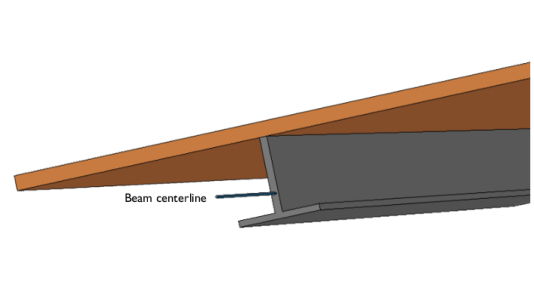
A beam can be coupled to a shell by adding a Shell-Beam Connection multiphysics coupling with Connection type set to either Shared boundaries or Parallel boundaries. This connection is used for adding beams as stiffeners to shells. The edges may be coincident or parallel. It is possible to prescribe that the beam has an offset from the shell when a coincident edge is used.

A beam can be coupled to a shell by adding a Shell-Beam Connection multiphysics coupling with Connection type set to Shell boundaries to beam points. This connection is used for modeling a beam with one end “welded” to the face of the shell. You can specify the size of the area on the shell boundary that is connected to the end point of the beam in several different ways.

A beam can be coupled to a shell by adding a Shell-Beam Connection multiphysics coupling with Connection type set to Shell edges to beam points. This connection is used for modeling a beam with one end “welded” to the edge of the shell. You can specify the part of the shell edge that is connected to the end point of the beam in several different ways.

A pipe in 3D can be coupled to a solid by adding a Structure-Pipe Connection multiphysics coupling. The coupling is intended for modeling a transition from a pipe to a solid where beam assumptions are valid on both sides of the connection. Thus, the geometry of the solid at the transition should match the cross-section data given to the pipe. The connection assumes that the pipe cross section is circular; if another cross section is used, it is converted to an equivalent circular cross section. This means that warping is not considered.

The connection can be considered an extension of the Solid boundaries to beam points, transition coupling in Solid-Beam Connection to also account for radial deformation of the pipe caused by the fluid pressure and the temperature difference over the cross section.

A pipe in 3D can be coupled to a shell by adding a Structure-Pipe Connection multiphysics coupling. The coupling is intended for modeling a transition from a pipe to a shell where beam assumptions are valid on both sides of the connection. Thus, the geometry of the shell at the transition should match the cross-section data given to the pipe. The connection assumes that the pipe cross section is circular; if another cross section is used, it is converted to an equivalent circular cross section. This means that warping is not considered.

The connection can be considered an extension of the Shell edges to beam points coupling in Shell-Beam Connection to also account for radial deformation of the pipe caused by the fluid pressure and the temperature difference over the cross section.

Lower dimension structural elements can be connected to a solid domain by adding an Embedded Reinforcement multiphysics coupling. This connection supports coupling truss, beam, and membrane elements to a Solid Mechanics interface. The connection can either be rigid, or made by attaching springs between points on the embedded structure and points in the solid. A more detailed discussion about this type of modeling is given in Modeling Embedded Structures and Reinforcements.

The most general method of connecting parts modeled with different physics interfaces is by using a General Extrusion operator. In this case the parts need not even be in contact, so the connection is an abstraction.

An example could be a shell stiffened by beams. In practice, you would probably use the built-in coupling described in Beam Edge to Shell Edge (3D) for this case, but the example shows the principles.

Here, is the rotation vector, which contains the rotational degrees of freedom in the Beam interface. The rotation vector is also available as a variable in the Shell interface, where it is derived from the rotational degrees of freedom a. The shell normal is denoted by n. Small rotations are assumed.