The distribution of dopants within the semiconductor can be specified using the Analytic Doping Model and Geometric Doping Model features. The Analytic Doping Model enables distributions to be defined in terms of the coordinate system; the Geometric Doping Model enables definitions in terms of the distance from selected boundaries in the geometry.

The Analytic Doping Model has two options to specify the doping concentration in terms of the coordinate system — User defined or Box. It supports the use of a local coordinate system that is rotated relative to the global coordinates.

The distribution outside of the constant region decays with one of three preset functions: Gaussian, Linear, or Error Function. These functions are defined using Ramp functions with unity gradient that begin at the edges of the constant region and which continue throughout the remainder of the domain. Thus there are two Ramp functions for each geometry axis. Figure 3-6 shows the four Ramp functions used to create a 2D Box profile. Note how each Ramp function is zero inside the constant region, and that the unity gradient outside the region creates and effective coordinate axis for each direction that is zeroed at the region boundary.

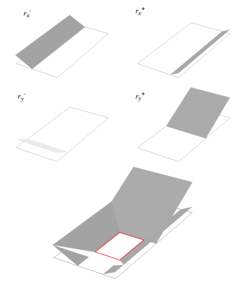
where Nd,a is the donor or acceptor concentration, N0 is the concentration inside the uniformly doped region, li is the Decay length in the i direction, and rx-, rx+, ry-, ry+, rz-, and rz+ are the Ramp functions.

where dj,i is the junction depth in the i direction, and Nb is the background doping concentration that can be entered directly or taken from the output of another doping feature in the model. By default dj,x=dj,y=dj,z=dj, such that lx=ly=lz. To use different decay lengths in different directions select the Specify different length scales for each direction check box under the Profile section.

where gi is the gradient in i direction. The gradient can be supplied directly or calculated from a specified junction depth via:

By default the gradient is the same in all directions, however it can be set to be direction dependent using the Specify different length scales for each direction check box. Note that a negative dopant distribution is not physical, so the concentration is set to zero in regions where Equation 3-44 gives Na,d<0.

where mx is an argument factor which controls the length scale of the profile. The argument factor can be entered directly or calculated from a specified junction depth via:

By default the argument factor is the same in all directions, however it can be set to be direction dependent using the Specify different length scales for each direction check box.

The Geometric Doping Model feature enables doping distributions to be defined in terms of the distance from selected boundaries in the geometry. This is convenient when working with geometries with intricate shapes that would be challenging to describe analytically using the coordinate system. The boundaries from which the distance is calculated are selected using the Boundary Selection for Doping Profile node. Any boundary that bounds, or is within, the domains to which the corresponding Geometric Doping Model feature is applied can be selected. The form of the distribution can be selected from a range of preset functions or a user defined expression can be supplied.

When a user defined profile is selected any arbitrary distribution that can be written in terms of the distance from the selected boundaries can be defined. This distance is available as the variable semi.gdm#.D, where # corresponds to the number of the Geometric Doping Model feature.

The other selections in the Dopant profile away from the boundary list allow either Gaussian, Linear, or Error Function profiles to be generated. These profiles are defined in terms of the distance, D, from the selected boundaries as described below.

where Nb is a specified background doping concentration that can either be directly defined or taken from the output of another doping model feature.

where g is the gradient, which can be entered directly or calculated from a specified junction depth via

Note that, as a negative concentration is not physical, the dopant concentration is set to zero in regions where Equation 3-45 gives Na,d<0.

where m is an argument factor which controls the length scale of the profile. The argument factor can be defined directly or calculated from a specified junction depth via: