|
|
|
|
The following example is similar to the model Bipolar Transistor, which is available in the Semiconductor Applications Libraries (Semiconductor_Module/Devices/bipolar_transistor).
|
|
1
|
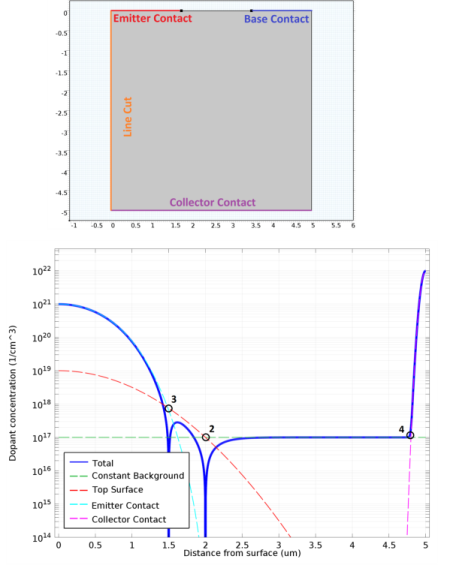
Constant background: a constant n-type doping of 1017 cm−3 is added using an Analytic Doping Model that specifies a User defined profile with constant Donor Concentration.
|
|
2
|
Top surface: a Box dopant distribution that decays away from the top surface with a Gaussian profile is added using a second Analytical Doping Model. The uniformly doped region is set to cover the entire width of the model at the top surface but to have zero depth, thus the profile decays away from the surface.
|
|
-
|
|
-
|
The donor concentration defined in the previous step, semi.adm1.Nd, is selected for the Background doping concentration.
|
|
-
|
The Junction depth is set to 2 μm below the top surface. Since the background doping is of a different type, semi.adm2.Na has equal magnitude to semi.adm1.Nd at this depth, as indicated by point 2 shown in Figure 2-6. Thus the overall contribution to semi.Nd-semi.Na due to the first two distributions is zero at a depth of 2 μm. This is an example of doping distribution into a constant background distribution of the opposite type.
|
|
3
|
Emitter contact: a Geometric Doping Model is used to define a Gaussian profile which decays away from the emitter contact.
|
|
-
|
The boundary that represents the emitter contact is selected in Boundary Selection for Doping Profile node and a Gaussian Dopant profile away from the boundary is selected.
|
|
-
|
|
-
|
The Background doping concentration must account for the effect of both of the two preceding steps. To achieve this, choose a User defined background concentration and set it to semi.adm2.Na-semi.adm1.Nd. This causes the resulting distribution, semi.gdm1.Nd, to be equal magnitude to semi.adm2.Na at the desired junction depth of 1.5 μm, as can be seen at point 3 labeled in Figure 2-6.
|
|
4
|
Collector contact: another Box distribution is defined with a third Analytic Doping Model. This is used to create a Gaussian profile that decays away from the collector contact. The uniformly doped region is set to cover the entire width of the model at the bottom surface but to have zero depth.
|
|
-
|
|
-
|
The Junction depth is set to 0.2 μm, which produces a junction at a depth of 4.8 μm from the top surface.
|
|
-
|
In this case the constant donor concentration defined in step 1 (1017 cm−3), semi.adm1.Nd, is selected for the Background doping concentration. Since donors are being doped into donors the concentration due to this final distribution (semi.adm3.Nd) is 2·1017 cm−3 at the junction depth, which is double the background level as indicated a point 4 shown in Figure 2-6. This is because at the junction depth semi.adm3.Nd has equal magnitude to the constant background and, because it is the same doping type, the sum of the contribution from both distributions results in double the concentration. This is an example of doping one type into a constant background of the same type.
|