The Geometric Doping Model enables doping profiles to be expressed as a function of the distance from selected boundaries. This is suitable for cases where the profile wanted is more conveniently expressed in terms of the geometry than the coordinate axes. The boundaries from which the distance is calculated using the Boundary Selection for Doping Profile node. The form of the profile is selected from the
Dopant profile away from the boundary list. This list contains preset functions that enable several common profiles to be easily defined. A
User defined option is also available that enables any expression to be manually entered.
A user-defined profile can be used to specify any dopant distribution that is expressed as a function of the distance from boundaries in the geometry. This distance is available as semi.gdm#.D within COMSOL, where
# indicates the number of the Geometric Doping Model feature.
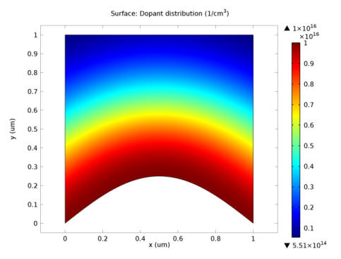
Figure 2-4 is an example doping profile that is created with the expression
1e16[1/cm^3]*exp(-(semi.gdm1.D/0.5[um])^2).
The Geometric Doping Model makes Gaussian, linear, and error function profiles available as options in the Dopant profile away from the boundary list. When a preset option is selected, the dopant concentration at the boundary can be input along with a parameter to set the decay length scale of the profile. The decay length scale of the profile is controlled by specifying a control length directly or by specifying a junction depth. The junction depth specifies the distance from the selected boundaries at which the dopant concentration is equal to the value specified in the
Background doping concentration user input.
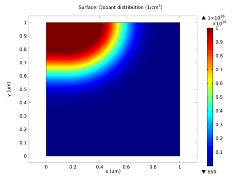
Figure 2-5 is an example profile that is created using a combination of an Analytic Doping Model and a Geometric Doping Model. The dopant concentration is constant within the top left domain, which is bounded by a curve. Away from this constant region the concentration decays with a Gaussian profile. The constant region is specified using a user-defined profile in an Analytic Doping Model. The Gaussian profile is achieved using a preset profile in a Geometric Doping Model with the curve as the selected boundary. This example shows how the Geometric Doping Model allows curves in the geometry to be easily incorporated into the dopant distribution, without the need to express the curves analytically in terms of the coordinate system.