Using the Analytic Doping Model
The Analytic Doping Model makes it possible to express doping profiles as a function of the local coordinate system, which can be rotated with respect to the global coordinate system if required. This is suitable to achieve profiles that are convenient to define in relation to the coordinate axes. The dopant distribution can be defined using either the user defined or box methods.
Analytic Doping Model: User defined
A user-defined doping distribution can be used to specify a constant dopant density in a domain. Alternately a spatially varying doping profile can be specified; the doping profile is defined using the functions available within COMSOL Multiphysics. Any analytic expression, written in terms of the local coordinate system, is permitted. FigureĀ 2-2 shows an example of a user-defined profile consisting of a Gaussian decay away from the lower boundary.
Doping distributions can also be imported from external files. This is useful when the required distribution cannot be defined analytically; for example, if the doping profile is output from an external diffusion simulation.
To import a doping profile using an interpolation function:
1
From the Definitions toolbar, click Interpolation ().
2
On the Settings window for Interpolation select File as the Data source.
3
Specify the Filename and the Number of arguments.
4
Once an interpolation function is defined, it can be used in an Analytical Doping Model feature. This is achieved by selecting a User defined dopant distribution and calling the interpolation function with the appropriate arguments.
Interpolation in the COMSOL Multiphysics Reference Manual.
Figure 2-2: Example of a user-defined dopant distribution created using the Analytic Doping Model feature. The Analytic Doping Model feature is the appropriate doping feature as this distribution is trivial to express as a function of the coordinate axes.
Analytic Doping Model: Box
The box method allows a block-shaped region of constant doping to be defined, along with a decay profile away from the region. This is useful for approximating some physical doping techniques, such as diffusion processes, which distribute dopants away from regions of high concentration resulting in characteristic decay profiles. The location of the region is defined by specifying either the corner or center coordinate using the global coordinate system. If a local rotated coordinate system is used within the feature, the orientation of the block rotates around this specified coordinate. A profile is selected from the Dopant profile away from uniform region list. The decay length scale of the profile is controlled by either specifying a control length directly or by specifying a junction depth. The junction depth specifies the distance, from the boundary of the uniformly doped region, where the dopant concentration is equal to the value specified in the Background doping concentration input. This distance can be specified independently for each axis in the component geometry by selecting Specify different length scales for each direction.
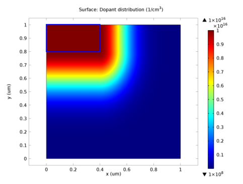
 FigureĀ 2-3 is an example of a doping profile created using this method. A rectangular region of uniform doping is specified in the top left of the geometry, and a Gaussian profile is selected away from this region with different junction depths in the x and y directions.
Figure 2-3: Example of a box doping distribution created using the Analytic Doping Model feature. This distribution is defined as a rectangle of constant doping located in the top left of the domain with a Gaussian decay profile away from the boundaries of this region. The region of uniform doping in the top left is outlined with a blue box.