PDF

Single Mode Fiber-to-Fiber Coupling
Introduction
Optical fibers can be used to efficiently transmit optical signals over large distances with minimal losses. Among the wide variety of fibers that exist, one important categorization criterion is if the fiber is multimode or single mode. In a single mode fiber, only one spatial mode can exist. Radiation profiles that don’t match that mode’s profile will not be bound to the core and, thus, have high losses. As the name already suggests, a multimode fiber, on the other hand, can support a set of spatial modes that can be transmitted almost without loss. For step index fibers, if the fiber or waveguide parameter
is below 2.405 only one spatial mode is supported. Here, n is the refractive index, a is the radius of the fiber core, and λ is the vacuum wavelength.
A common way to couple light into an optical fiber is to start with a free space beam and use a lens to focus the light onto the fiber end. When a light field enters a fiber, it is decomposed into the set of modes that can exist in the fiber. As the fibers are mode-selective, we have to make sure that the mode impinging onto the fiber tip will be coupled in to the fiber. In the case of a single mode fiber, where only one spatial mode is guided, the input beam has to match this one specific mode of the fiber. The field emitted by the fiber is the proper input field on the fiber. Field components in other spatial modes will be lost in the cladding as they are not guided.
Model Definition
This model uses the Electromagnetic Waves, Beam Envelopes interface in the unidirectional formulation to model the free space fiber-to-fiber coupling with two identical lenses. The first lens collimates the light emitted by the fiber, while the second lens focuses the collimated light onto the second fiber tip. The unidirectional formulation is a good choice, as all surfaces in this model use single layer anti-reflective coatings to suppress reflections. The geometry is surrounded by Perfectly Matched Layers to absorb any outgoing waves.
The anti-reflection (AR) coatings between air with n = 1 and a material with refractive index nmat are defined using a Transition Boundary Condition that models a thin layer with refractive index and thickness .
At the fiber tips, the computed effective mode index ewbe.neff_1 is used when calculating the refractive index of the AR coating. As both fibers are identical, ewbe.neff_1 = ewbe.neff_2.
To reduce the necessary number of mesh elements along the optical axis and make efficient use of the beam envelopes method, proper choice of the phase function is crucial. Here, the different domains are assigned local phase functions. In the fibers, the propagation constant ewbe.beta_1 is solved for in a Boundary Mode Analysis study step. Thus, here the phase is defined as ewbe.beta_1*x. In the air domain and the lenses, the local free-space propagation constant ewbe.k is used. For these domains, the phase is defined as ewbe.k*x. Normally, the phase function should be continuous everywhere. However, the Transition Boundary Condition allows the user-defined phase function to be discontinuous and, thus, different local phase functions can be used, as described above.
The key metric we want to analyze in this model is the fiber-to-fiber coupling efficiency. How much of the light that is guided in the first fiber will be coupled into the (identical) mode of the second fiber? To compute this value, we use two Ports of the Numeric type in the model. The Boundary Mode Analysis study steps, compute the eigenmodes and propagation constants of the fibers. The final Frequency Domain study step, solves for the electric field in the domains and the S-parameters. The port on the right-hand side is a Slit Port, which allows it to be defined on an internal boundary, backed by a Perfectly Matched Layer (PML). Here, the S-parameter is calculated as the overlap of the input field and the fiber mode. The PML-backed Slit Port makes sure that all outgoing radiation is absorbed. If a Slit Port would not be used, only the fiber (Port) mode would be absorbed and reflections would occur for all field components that are not matching the particular fiber (Port) mode.
To find the proper lens position, the second lens is moved with a Parametric Sweep and the total transmission is analyzed.
Results and Discussion
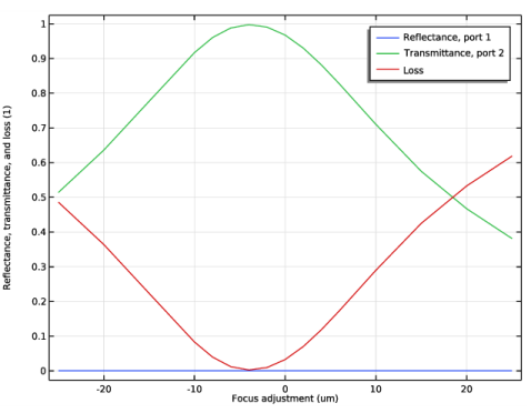
Figure 1 shows that the coupling loss is minimized when the lenses are moved 4 μm closer to the fiber ends than the nominal focal length of the lens.
Figure 1: The plot shows the reflectance (blue), transmittance (green), and loss (red) for the fiber-to-fiber coupling system. As shown, the loss is minimized when the lenses are moved 4 μm closer to the fiber end than the nominal focal length.
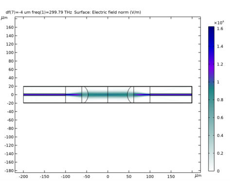
Figure 2 shows a field plot for the case when the lenses are located in the position for minimum coupling loss. It is clear from both Figure 1 and Figure 2 that the anti-reflection coatings, modeled using the Transition boundary condition, eliminate the reflections at the fiber ends and at the lens surfaces. Thus, justifying the use of the unidirectional formulation.
Figure 2: The norm of the electric field, when the lenses are in the position for minimum losses.
Application Library path: Wave_Optics_Module/Waveguides_and_Couplers/single_mode_fiber_coupling
Modeling Instructions
From the File menu, choose New.
New
In the New window, click  Model Wizard.
Model Wizard
1
In the Model Wizard window, click  2D.
2
In the Select Physics tree, select Optics>Wave Optics>Electromagnetic Waves, Beam Envelopes (ewbe).
3
Click Add.
4
Click  Study.
5
In the Select Study tree, select Preset Studies for Selected Physics Interfaces>Boundary Mode Analysis.
6
Global Definitions
Parameters 1
1
In the Model Builder window, under Global Definitions click Parameters 1.
2
In the Settings window for Parameters, locate the Parameters section.
3
Click  Load from File.
4
Geometry 1
1
In the Model Builder window, under Component 1 (comp1) click Geometry 1.
2
In the Settings window for Geometry, locate the Units section.
3
From the Length unit list, choose µm.
Rectangle 1 (r1)
1
In the Geometry toolbar, click  Rectangle.
2
In the Settings window for Rectangle, locate the Size and Shape section.
3
In the Width text field, type l_fiber.
4
In the Height text field, type h_core.
5
Locate the Position section. From the Base list, choose Center.
6
In the x text field, type -l_fiber/2-l_dom.
Rectangle 2 (r2)
1
Right-click Rectangle 1 (r1) and choose Duplicate.
2
In the Settings window for Rectangle, locate the Size and Shape section.
3
In the Height text field, type h_clad.
4
Click to expand the Layers section. In the table, enter the following settings:
5
Select the Layers on top check box. The Layers on bottom check box is selected by default.
Rectangle 3 (r3)
1
In the Geometry toolbar, click  Rectangle.
2
In the Settings window for Rectangle, locate the Size and Shape section.
3
In the Width text field, type l_dom.
4
In the Height text field, type h_clad.
5
Locate the Position section. In the x text field, type -l_dom.
6
In the y text field, type -h_clad/2.
7
Locate the Layers section. In the table, enter the following settings:
8
Select the Layers on top check box.
9
Click  Build Selected.
10
Click the  Zoom Extents button in the Graphics toolbar.
Circle 1 (c1)
1
In the Geometry toolbar, click  Circle.
2
In the Settings window for Circle, locate the Size and Shape section.
3
In the Radius text field, type r_lens.
4
Locate the Position section. In the x text field, type r_lens.
Rectangle 4 (r4)
1
In the Geometry toolbar, click  Rectangle.
2
In the Settings window for Rectangle, locate the Size and Shape section.
3
In the Width text field, type t_lens-(r_lens-sqrt(r_lens^2-h_clad^2/4)).
4
In the Height text field, type h_clad.
5
Locate the Position section. In the x text field, type r_lens-sqrt(r_lens^2-h_clad^2/4).
6
In the y text field, type -h_clad/2.
7
Click  Build Selected.
8
Click the  Zoom Extents button in the Graphics toolbar.
Union 1 (uni1)
1
In the Geometry toolbar, click  Booleans and Partitions and choose Union.
2
Select the objects c1 and r4 only.
Delete Entities 1 (del1)
1
In the Model Builder window, right-click Geometry 1 and choose Delete Entities.
2
In the Settings window for Delete Entities, locate the Entities or Objects to Delete section.
3
From the Geometric entity level list, choose Domain.
4
On the object uni1, select Domain 3 only.
Union 2 (uni2)
1
In the Geometry toolbar, click  Booleans and Partitions and choose Union.
2
3
In the Settings window for Union, locate the Union section.
4
Clear the Keep interior boundaries check box.
Rotate 1 (rot1)
1
In the Geometry toolbar, click  Transforms and choose Rotate.
2
3
In the Settings window for Rotate, locate the Rotation section.
4
In the Angle text field, type 180.
Move 1 (mov1)
1
In the Geometry toolbar, click  Transforms and choose Move.
2
3
In the Settings window for Move, locate the Displacement section.
4
In the x text field, type -t_lens/2+f_lens+df-l_dom+t_lens.
5
Click  Build Selected.
Mirror 1 (mir1)
1
In the Geometry toolbar, click  Transforms and choose Mirror.
2
Click the  Select All button in the Graphics toolbar.
3
In the Settings window for Mirror, locate the Input section.
4
Select the Keep input objects check box.
5
Click  Build Selected.
6
Click the  Zoom Extents button in the Graphics toolbar.
Rectangle 5 (r5)
1
In the Geometry toolbar, click  Rectangle.
2
In the Settings window for Rectangle, locate the Size and Shape section.
3
In the Width text field, type t_PML.
4
In the Height text field, type h_clad.
5
Locate the Position section. In the x text field, type l_dom+l_fiber-t_PML.
6
In the y text field, type -h_clad/2.
7
Click  Build All Objects.
Materials
Air
1
In the Model Builder window, under Component 1 (comp1) right-click Materials and choose Blank Material.
2
In the Settings window for Material, type Air in the Label text field.
3
Locate the Material Contents section. In the table, enter the following settings:
Lens
1
Right-click Materials and choose Blank Material.
2
In the Settings window for Material, type Lens in the Label text field.
3
4
Locate the Material Contents section. In the table, enter the following settings:
Core
1
Right-click Materials and choose Blank Material.
2
In the Settings window for Material, type Core in the Label text field.
3
4
Locate the Material Contents section. In the table, enter the following settings:
Cladding
1
Right-click Materials and choose Blank Material.
2
In the Settings window for Material, type Cladding in the Label text field.
3
4
Locate the Material Contents section. In the table, enter the following settings:
Electromagnetic Waves, Beam Envelopes (ewbe)
1
In the Model Builder window, under Component 1 (comp1) click Electromagnetic Waves, Beam Envelopes (ewbe).
2
In the Settings window for Electromagnetic Waves, Beam Envelopes, locate the Components section.
3
From the Electric field components solved for list, choose Out-of-plane vector.
4
Locate the Wave Vectors section. From the Number of directions list, choose Unidirectional.
5
From the Type of phase specification list, choose User defined.
6
In the φ1 text field, type psi. This variable will be defined after all physics features have been added.
Port 1
1
In the Physics toolbar, click  Boundaries and choose Port.
2
3
In the Settings window for Port, locate the Port Properties section.
4
From the Type of port list, choose Numeric.
Port 2
1
In the Physics toolbar, click  Boundaries and choose Port.
2
3
In the Settings window for Port, locate the Port Properties section.
4
From the Type of port list, choose Numeric.
5
Select the Activate slit condition on interior port check box.
6
From the Slit type list, choose Domain-backed.
Transition Boundary Condition 1
Now, add a Transition boundary condition feature, to model anti-reflection (AR) coatings on the fiber ends.
1
In the Physics toolbar, click  Boundaries and choose Transition Boundary Condition.
2
3
In the Settings window for Transition Boundary Condition, locate the Transition Boundary Condition section.
4
From the n list, choose User defined. In the associated text field, type sqrt(ewbe.neff_1), to define the refractive index for the AR coating layer.
5
From the k list, choose User defined. In the d text field, type lda0/4/sqrt(ewbe.neff_1), to define the thickness of the AR coating layer.
Transition Boundary Condition 2
Next, add a Transition boundary condition feature, to model AR coatings on the lens surfaces.
1
In the Physics toolbar, click  Boundaries and choose Transition Boundary Condition.
2
3
In the Settings window for Transition Boundary Condition, locate the Transition Boundary Condition section.
4
From the n list, choose User defined. In the associated text field, type sqrt(n_lens).
5
From the k list, choose User defined. In the d text field, type lda0/4/sqrt(n_lens).
Definitions
Now, add expressions for the user-defined phase, that is used by the Electromagnetic Waves, Beam Envelopes interface.
Variables 1
1
In the Model Builder window, under Component 1 (comp1) right-click Definitions and choose Variables.
2
In the Settings window for Variables, locate the Geometric Entity Selection section.
3
From the Geometric entity level list, choose Domain.
4
5
Locate the Variables section. In the table, enter the following settings:
Variables 2
1
In the Model Builder window, right-click Definitions and choose Variables.
2
In the Settings window for Variables, locate the Geometric Entity Selection section.
3
From the Geometric entity level list, choose Domain.
4
5
Locate the Variables section. In the table, enter the following settings:
Perfectly Matched Layer 1 (pml1)
1
In the Definitions toolbar, click  Perfectly Matched Layer.
2
Mesh 1
Define a mesh that resolves the variations of the field envelope.
1
In the Model Builder window, under Component 1 (comp1) right-click Mesh 1 and choose Build All.
2
In the Settings window for Mesh, locate the Sequence Type section.
3
From the list, choose User-controlled mesh.
Distribution - Air Space
1
In the Model Builder window, under Component 1 (comp1)>Mesh 1 click Distribution 1.
2
In the Settings window for Distribution, type Distribution - Air Space in the Label text field.
3
Locate the Boundary Selection section. Click  Clear Selection.
4
5
Locate the Distribution section. In the Number of elements text field, type 15.
Distribution - Core
1
In the Model Builder window, under Component 1 (comp1)>Mesh 1 click Distribution 2.
2
In the Settings window for Distribution, type Distribution - Core in the Label text field.
3
Locate the Boundary Selection section. Click  Clear Selection.
4
5
Locate the Distribution section. In the Number of elements text field, type 22.
Distribution - Cladding
1
In the Model Builder window, under Component 1 (comp1)>Mesh 1 click Distribution 3.
2
In the Settings window for Distribution, type Distribution - Cladding in the Label text field.
3
Locate the Boundary Selection section. Click  Clear Selection.
4
5
Locate the Distribution section. In the Number of elements text field, type 80.
Distribution - PML
1
In the Model Builder window, right-click Mesh 1 and choose Distribution.
2
In the Settings window for Distribution, type Distribution - PML in the Label text field.
3
Locate the Boundary Selection section. Click  Clear Selection.
4
5
Locate the Distribution section. In the Number of elements text field, type 10.
6
Right-click Distribution - PML and choose Move Up.
Distribution - Input Fiber
1
In the Model Builder window, right-click Mesh 1 and choose Distribution.
2
In the Settings window for Distribution, type Distribution - Input Fiber in the Label text field.
3
4
Locate the Distribution section. In the Number of elements text field, type 10.
Distribution - Output Fiber
1
Right-click Mesh 1 and choose Distribution.
2
In the Settings window for Distribution, type Distribution - Output Fiber in the Label text field.
3
4
Locate the Distribution section. In the Number of elements text field, type 20.
Distribution - Lens
1
Right-click Mesh 1 and choose Distribution.
2
In the Settings window for Distribution, type Distribution - Lens in the Label text field.
3
4
Click  Build All.
Study 1
Step 1: Boundary Mode Analysis
1
In the Model Builder window, under Study 1 click Step 1: Boundary Mode Analysis.
2
In the Settings window for Boundary Mode Analysis, locate the Study Settings section.
3
In the Mode analysis frequency text field, type f0.
4
Select the Search for modes around check box.
5
Step 3: Boundary Mode Analysis 1
1
Right-click Study 1>Step 1: Boundary Mode Analysis and choose Duplicate.
2
In the Settings window for Boundary Mode Analysis, locate the Study Settings section.
3
In the Port name text field, type 2.
4
Right-click Step 3: Boundary Mode Analysis 1 and choose Move Up.
Step 3: Frequency Domain
1
In the Model Builder window, click Step 3: Frequency Domain.
2
In the Settings window for Frequency Domain, locate the Study Settings section.
3
In the Frequencies text field, type f0.
Parametric Sweep
1
In the Study toolbar, click  Parametric Sweep.
2
In the Settings window for Parametric Sweep, locate the Study Settings section.
3
4
5
6
In the Study toolbar, click  Compute.
Results
In the default reflectance and transmittance plot, replace the term absorptance everywhere with loss, as reflectance and transmittance here refer to what is reflected back into the guided mode of the input fiber and what is coupled into the guided mode of the output fiber, respectively. The light that is not transmitted to the guided mode of the output fiber is not absorbed by any material, but lost to radiation modes other than the guided mode of the output fiber.
Reflectance, Transmittance, and Loss(ewbe)
1
In the Model Builder window, under Results click Reflectance, Transmittance, and Absorptance (ewbe).
2
In the Settings window for 1D Plot Group, type Reflectance, Transmittance, and Loss(ewbe) in the Label text field.
3
Locate the Plot Settings section. In the y-axis label text field, type Reflectance, transmittance, and loss (1).
Global 1
1
In the Model Builder window, expand the Reflectance, Transmittance, and Loss(ewbe) node, then click Global 1.
2
In the Settings window for Global, locate the y-Axis Data section.
3
4
Click  Delete, to delete the less interesting variable representing the total transmittance and reflectance.
Replace also the description for the Absorptance variable with Loss.
5
6
In the Reflectance, Transmittance, and Loss(ewbe) toolbar, click  Plot.
The coupling loss can be obtained from the plot above. The minimum value is found when the lenses are 4 μm closer to the fiber ends than the nominal focal length.
Electric Field (ewbe)
Now, plot the field under conditions of maximum fiber-to-fiber coupling.
1
In the Model Builder window, under Results click Electric Field (ewbe).
2
In the Settings window for 2D Plot Group, locate the Data section.
3
From the Parameter value (df (um)) list, choose -4.
Electric Field
1
In the Model Builder window, expand the Electric Field (ewbe) node, then click Electric Field.
2
In the Settings window for Surface, locate the Coloring and Style section.
3
From the Color table list, choose AuroraAustralis.
4
In the Electric Field (ewbe) toolbar, click  Plot.
Now inspect the mode field plot and the effective mode index resulting from the boundary mode analysis performed for each port.
Electric Mode Field, Port 1 (ewbe)
Electric Mode Field, Port 2 (ewbe)