PDF

Optical Scattering off a Gold Nanosphere
Introduction
This model demonstrates the calculation of the scattering of a plane wave of light off a gold nanosphere. The scattering is computed for the optical frequency range, over which gold can be modeled as a material with negative complex-valued permittivity. The far-field pattern and the losses are computed.
Figure 1: A gold sphere illuminated by a plane wave. Due to symmetry, only one-quarter of the sphere has to be modeled.
Model Definition
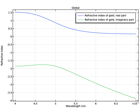
A gold sphere of radius r = 100 nm is illuminated by a plane wave, as shown in Figure 1. The free space wavelength range from 400 nm to 700 nm is simulated. The complex refractive index of gold is taken from the Optical Materials Database, where interpolation functions for a large number of commonly used optical materials are found. Figure 2 shows the real and the imaginary parts of the refractive index for gold, for the wavelength range used in the simulation.
Figure 2: The real and the imaginary parts of the refractive index for gold.
From the refractive index, the relative permittivity is found from the relation
,
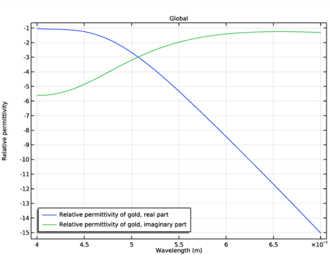
where the real parts of the relative permittivity and the refractive index are denoted with primes and, similarly, the imaginary parts are denoted with bis. Figure 3 shows the relative permittivity, corresponding to the refractive index plotted in Figure 2. Notice that the real part of the relative permittivity is negative for this wavelength range.
Figure 3: The real and the imaginary parts of the relative permittivity of gold.
Over the wavelength range of interest, it is possible to compute the skin depth via
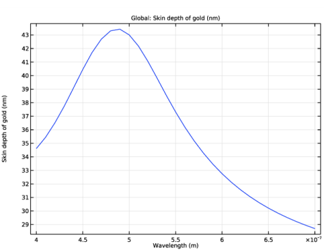
where k0 is the free space wave number, and εr is the complex-valued relative permittivity. The skin depth is shown in Figure 4, and ranges from 28 nm to 44 nm. The skin depth is evaluated with assumption of plane wave incidence over flat surface, so it is not directly applicable on the gold sphere in the model.
Figure 4: The skin depth of gold.
Due to the symmetry of the problem, only one-quarter of the sphere is modeled. A region of air around the sphere is also modeled, of width equal to half the wavelength in free space. A perfectly matched layer (PML) domain is outside of the air domain and acts as an absorber of the scattered field. The PML should not be within the reactive near-field of the scatterer, placing it a half-wavelength away is usually sufficient. The far-field radiation pattern and the heat losses are computed.
Results and Discussion
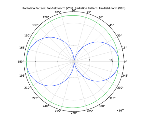
The far-field patterns show that, at short wavelengths, a single gold sphere scatters light forward, in the direction of propagation of the incident light. At longer wavelengths, the scattered fields from the sphere look more as the radiation pattern of a dipole antenna. The far-field radiation pattern for a wavelength of 700 nm is plotted in Figure 5. The E-plane and H-plane notation originates from antenna theory, where the E-plane denotes the plane containing the electric field polarization and the direction of maximum radiation, whereas the H-plane denotes the plane containing the magnetic field and the direction of maximum radiation. In this case, the E-plane denotes the xz-plane and the H-plane denotes the xy-plane.
The heat losses, plotted in Figure 6, show that the particle preferentially absorbs the shorter wavelengths. The radius of the sphere can also be varied to see how the absorption depends upon the geometry.
Figure 5: The far-field radiation pattern in the E-plane (blue) and H-plane (green) when wavelength is 700 nm.
Figure 6: The resistive heating losses in the gold sphere.
Application Library path: Wave_Optics_Module/Optical_Scattering/scattering_nanosphere
Modeling Instructions
From the File menu, choose New.
New
In the New window, click  Model Wizard.
Model Wizard
1
In the Model Wizard window, click  3D.
2
In the Select Physics tree, select Optics>Wave Optics>Electromagnetic Waves, Frequency Domain (ewfd).
3
Click Add.
4
Click  Study.
5
In the Select Study tree, select Preset Studies for Selected Physics Interfaces>Wavelength Domain.
6
Global Definitions
Define some parameters that are useful for setting up the geometry and the study.
Parameters 1
1
In the Model Builder window, under Global Definitions click Parameters 1.
2
In the Settings window for Parameters, locate the Parameters section.
3
Here, c_const is a predefined COMSOL constant for the speed of light.
Geometry 1
Create a sphere with layers. The outermost layer represents the PMLs and the core represents the gold sphere. The middle layer is the air domain.
Sphere 1 (sph1)
1
In the Geometry toolbar, click  Sphere.
2
In the Settings window for Sphere, locate the Size section.
3
In the Radius text field, type r0+t_air+t_pml.
4
Click to expand the Layers section. In the table, enter the following settings:
5
Click  Build Selected.
Choose wireframe rendering to get a better view of the interior parts.
6
Click the  Wireframe Rendering button in the Graphics toolbar.
Block 1 (blk1)
Then, add a block intersecting one-quarter of the sphere.
1
In the Geometry toolbar, click  Block.
2
In the Settings window for Block, locate the Size and Shape section.
3
In the Width text field, type 2*(r0+t_air+t_pml).
4
In the Depth text field, type 2*(r0+t_air+t_pml).
5
In the Height text field, type 2*(r0+t_air+t_pml).
6
Locate the Position section. In the x text field, type -(r0+t_air+t_pml).
7
Click  Build Selected.
Intersection 1 (int1)
Generate the quarter sphere by intersecting two objects.
1
In the Geometry toolbar, click  Booleans and Partitions and choose Intersection.
2
Click in the Graphics window and then press Ctrl+A to select both objects.
3
In the Settings window for Intersection, click  Build All Objects.
4
Click the  Zoom Extents button in the Graphics toolbar.
Definitions
Add a variable for the total heat losses in the gold sphere computed as a volume integral of resistive losses. First, add a nonlocal integration coupling for the volume integral of the gold sphere.
Integration 1 (intop1)
1
In the Definitions toolbar, click  Nonlocal Couplings and choose Integration.
2
In the Settings window for Integration, type int_L in the Operator name text field.
3
Variables 1
1
In the Definitions toolbar, click  Local Variables.
Add the heat loss variable for gold and variables representing the refractive index, the relative permittivity, and the skin depth of gold.
2
In the Settings window for Variables, locate the Variables section.
3
Here, the ewfd. prefix gives the correct physics-interface scope for the resistive losses. By calculating the average refractive index for the gold sphere, this averaged variable can later be evaluated in a global plot.
Materials
Assign air as the material for all domains, except for the gold sphere.
Add Material
1
In the Home toolbar, click  Add Material to open the Add Material window.
2
Go to the Add Material window.
3
4
Click Add to Component in the window toolbar.
5
In the tree, select Optical>Inorganic Materials>Au - Gold>Models and simulations>Au (Gold) (Rakic et al. 1998: Brendel-Bormann model; n,k 0.248-6.20 um).
6
Click Add to Component in the window toolbar.
7
In the Home toolbar, click  Add Material to close the Add Material window.
Materials
Au (Gold) (Rakic et al. 1998: Brendel-Bormann model; n,k 0.248-6.20 um) (mat2)
Select Domain 3 only.
Electromagnetic Waves, Frequency Domain (ewfd)
Now set up the physics. You solve the model for the scattered field, so it needs background electric field (E-field) information. The background plane wave is traveling in the positive x direction, with the electric field polarized along the z-axis. The default boundary condition is perfect electric conductor, which applies to all exterior boundaries including the boundaries perpendicular to the background E-field polarization.
1
In the Model Builder window, under Component 1 (comp1) click Electromagnetic Waves, Frequency Domain (ewfd).
2
In the Settings window for Electromagnetic Waves, Frequency Domain, locate the Formulation section.
3
From the list, choose Scattered field.
4
Specify the Eb vector as
Scattering Boundary Condition 1
1
In the Physics toolbar, click  Boundaries and choose Scattering Boundary Condition.
2
Definitions
The outermost domains from the center of the sphere are the PMLs.
Perfectly Matched Layer 1 (pml1)
1
In the Definitions toolbar, click  Perfectly Matched Layer.
2
3
In the Settings window for Perfectly Matched Layer, locate the Geometry section.
4
From the Type list, choose Spherical.
Electromagnetic Waves, Frequency Domain (ewfd)
Set PMC on the boundaries parallel to the background E-field polarization.
Perfect Magnetic Conductor 1
1
In the Physics toolbar, click  Boundaries and choose Perfect Magnetic Conductor.
2
Far-Field Domain 1
In the Physics toolbar, click  Domains and choose Far-Field Domain.
Far-Field Calculation 1
1
In the Model Builder window, expand the Far-Field Domain 1 node, then click Far-Field Calculation 1.
2
In the Settings window for Far-Field Calculation, locate the Far-Field Calculation section.
3
Select the Symmetry in the y=0 plane check box.
4
Select the Symmetry in the z=0 plane check box.
5
From the Symmetry type list, choose Symmetry in H (PEC).
Mesh 1
Automatically define the mesh from the specified wavelength and the material parameters.
1
In the Model Builder window, under Component 1 (comp1) click Mesh 1.
2
In the Settings window for Mesh, locate the Electromagnetic Waves, Frequency Domain (ewfd) section.
3
From the Maximum mesh element size control parameter list, choose Wavelength.
4
In the Minimum vacuum wavelength text field, type lda.
5
Select the Resolve wave in lossy media check box, to resolve the field down to the skin depth in the gold sphere.
Study 1
Add a parametric sweep to create a new mesh for each wavelength in the sweep.
Parametric Sweep
1
In the Study toolbar, click  Parametric Sweep.
2
In the Settings window for Parametric Sweep, locate the Study Settings section.
3
4
Step 1: Wavelength Domain
1
In the Model Builder window, click Step 1: Wavelength Domain.
2
In the Settings window for Wavelength Domain, locate the Study Settings section.
3
In the Wavelengths text field, type lda.
4
In the Model Builder window, click Study 1.
5
In the Settings window for Study, locate the Study Settings section.
6
Clear the Generate default plots check box.
7
In the Study toolbar, click  Compute.
Results
Begin the results analysis and visualization by adding a selection to see the resistive losses only inside the gold sphere.
In the Model Builder window, expand the Results node.
Study 1/Parametric Solutions 1 (sol2)
In the Model Builder window, expand the Results>Datasets node, then click Study 1/Parametric Solutions 1 (sol2).
Selection
1
In the Results toolbar, click  Attributes and choose Selection.
2
In the Settings window for Selection, locate the Geometric Entity Selection section.
3
From the Geometric entity level list, choose Domain.
4
3D Plot Group 1
1
In the Results toolbar, click  3D Plot Group.
2
In the Settings window for 3D Plot Group, locate the Data section.
3
From the Dataset list, choose Study 1/Parametric Solutions 1 (sol2).
Volume 1
1
Right-click 3D Plot Group 1 and choose Volume.
2
In the Settings window for Volume, click Replace Expression in the upper-right corner of the Expression section. From the menu, choose Component 1 (comp1)>Electromagnetic Waves, Frequency Domain>Heating and losses>ewfd.Qrh - Resistive losses - W/m³.
3
In the 3D Plot Group 1 toolbar, click  Plot.
4
Click the  Zoom Extents button in the Graphics toolbar.
Polar Plot Group 2
The following instructions reproduce the polar plot of the far-field at the E-plane and H-plane shown in Figure 5.
1
In the Home toolbar, click  Add Plot Group and choose Polar Plot Group.
2
In the Settings window for Polar Plot Group, locate the Data section.
3
From the Dataset list, choose Study 1/Parametric Solutions 1 (sol2).
4
From the Parameter selection (lda) list, choose Last.
Radiation Pattern 1
1
In the Polar Plot Group 2 toolbar, click  More Plots and choose Radiation Pattern.
2
In the Settings window for Radiation Pattern, locate the Evaluation section.
3
Find the Angles subsection. In the Number of angles text field, type 100.
4
Find the Normal vector subsection. In the y text field, type 1.
5
In the z text field, type 0.
6
Click to expand the Legends section. From the Legends list, choose Manual.
7
8
In the Polar Plot Group 2 toolbar, click  Plot.
The E-plane in this model is located on the xz-plane where angle φ is measured counterclockwise from the x-axis.
Polar Plot Group 2
Add the H-plane polar plot.
In the Model Builder window, click Polar Plot Group 2.
Radiation Pattern 2
1
In the Polar Plot Group 2 toolbar, click  More Plots and choose Radiation Pattern.
2
In the Settings window for Radiation Pattern, locate the Evaluation section.
3
Find the Angles subsection. In the Number of angles text field, type 100.
4
Locate the Legends section. From the Legends list, choose Manual.
5
6
In the Polar Plot Group 2 toolbar, click  Plot.
1D Plot Group 3
The following instructions create a plot of the heat losses inside the gold sphere (see Figure 6).
1
In the Home toolbar, click  Add Plot Group and choose 1D Plot Group.
2
In the Settings window for 1D Plot Group, locate the Data section.
3
From the Dataset list, choose Study 1/Parametric Solutions 1 (sol2).
Global 1
1
Right-click 1D Plot Group 3 and choose Global.
2
In the Settings window for Global, click Replace Expression in the upper-right corner of the y-Axis Data section. From the menu, choose Component 1 (comp1)>Definitions>Variables>l_gold - Heat losses - W.
3
Locate the x-Axis Data section. From the Axis source data list, choose Outer solutions.
4
Click to expand the Legends section. Clear the Show legends check box.
1D Plot Group 3
1
In the Model Builder window, click 1D Plot Group 3.
2
In the Settings window for 1D Plot Group, locate the Plot Settings section.
3
Select the x-axis label check box.
4
5
In the 1D Plot Group 3 toolbar, click  Plot. Compare the resulting plot with Figure 6.
1D Plot Group 4
Finally, add plots showing the real and the imaginary parts of the refractive index and the relative permittivity of gold, as well as the skin depth.
1
Right-click Results>1D Plot Group 3 and choose Duplicate.
2
In the Settings window for 1D Plot Group, locate the Plot Settings section.
3
Select the y-axis label check box.
4
Global 1
1
In the Model Builder window, expand the 1D Plot Group 4 node, then click Global 1.
2
In the Settings window for Global, click Replace Expression in the upper-right corner of the y-Axis Data section. From the menu, choose Component 1 (comp1)>Definitions>Variables>n_gold - Refractive index of gold.
3
Locate the y-Axis Data section. In the table, enter the following settings:
4
Locate the Legends section. Select the Show legends check box.
5
From the Legends list, choose Manual.
6
7
In the 1D Plot Group 4 toolbar, click  Plot. Compare the resulting plot with Figure 2.
1D Plot Group 5
In the Model Builder window, under Results right-click 1D Plot Group 4 and choose Duplicate.
Global 1
1
In the Model Builder window, expand the 1D Plot Group 5 node, then click Global 1.
2
In the Settings window for Global, click Replace Expression in the upper-right corner of the y-Axis Data section. From the menu, choose Component 1 (comp1)>Definitions>Variables>epsilonr_gold - Relative permittivity of gold.
3
Locate the y-Axis Data section. In the table, enter the following settings:
4
Locate the Legends section. In the table, enter the following settings:
1D Plot Group 5
1
In the Model Builder window, click 1D Plot Group 5.
2
In the Settings window for 1D Plot Group, locate the Plot Settings section.
3
In the y-axis label text field, type Relative permittivity.
4
Locate the Legend section. From the Position list, choose Lower left.
5
In the 1D Plot Group 5 toolbar, click  Plot. Compare the resulting plot with Figure 3 and notice that the real part of the relative permittivity is negative in this wavelength range.
1D Plot Group 6
In the Model Builder window, under Results right-click 1D Plot Group 3 and choose Duplicate.
Global 1
1
In the Model Builder window, expand the 1D Plot Group 6 node, then click Global 1.
2
In the Settings window for Global, click Replace Expression in the upper-right corner of the y-Axis Data section. From the menu, choose Component 1 (comp1)>Definitions>Variables>deltaS_gold - Skin depth of gold - m.
3
Locate the y-Axis Data section. In the table, enter the following settings:
4
In the 1D Plot Group 6 toolbar, click  Plot. Compare the resulting plot with Figure 4.