PDF

Modeling a Negative Refractive Index
Introduction
It is possible to engineer the structure of materials such that both the permittivity and permeability are negative. Such materials are realized by engineering a periodic structure with features comparable in scale to the wavelength. It is possible to model both the individual unit cells of such a material, as well as to model to properties of a bulk negative index material. This example demonstrates the correct way to model a metamaterial domain with bulk negative permittivity and permeability.
Figure 1: A plane wave of light incident upon an infinite half-space of material with negative permittivity and permeability.
Model Definition
A plane wave (λ = 1 m) traveling through vacuum (εr 1, μr = 1) is incident at an angle of 30? upon an infinite half-space of metamaterial with bulk negative permittivity and permeability (εr = 1, μr = 1) as shown in Figure 1. The objective of the analysis is to observe the fields in the metamaterial.
Since the model space is infinite and invariant along the interface, it is possible to model a finite-sized unit cell around the interface, and use Floquet-periodic boundary conditions. The incident wave is modeled using a Port boundary condition, which both launches the incident wave and absorbs the reflected wave.
Two different ways are demonstrated for modeling boundary to the infinite metamaterial domain. In the first case, a Port boundary condition is used. This boundary condition requires computing the wave vector in the metamaterial, and manually adjusting the propagation constant at the boundary to account for the negative index. In the other case, a Perfectly Matched Layer (PML) is used to truncate the domain. The PML acts as an absorbing medium for all energy incident upon it, but must also be adjusted to account for the negative index. It is simpler to use, but increases the model size.
The transition between the two materials requires some special care. The natural boundary condition between domains of different material properties does not account for the change in direction of the flux. An additional degree of freedom has to be added to the model. This can be done by using the Transition Boundary Condition (TBC), which allows for a change in flux across the boundary. The TBC takes as input the material properties on one side of the domain, it does not matter which side. The thickness of the TBC should be approximately 1/1000 of the wavelength. If it is too small, it can introduce numerical difficulties. If it is too big, it alters the results significantly. The TBC only needs to be used in this way if the effective refractive index is similar in magnitude, but opposite in sign.
Results and Discussion
The electric field is plotted in Figure 2. The fields within the PML are not plotted, since these have no physical meaning. The wave is observed to switch direction at the interface between vacuum and the metamaterial.
Figure 2: The electric fields in vacuum and in the metamaterial. The waves are observed to switch direction.
Application Library path: Wave_Optics_Module/Gratings_and_Metamaterials/negative_refractive_index
Modeling Instructions
From the File menu, choose New.
New
In the New window, click  Model Wizard.
Model Wizard
1
In the Model Wizard window, click  2D.
2
In the Select Physics tree, select Optics>Wave Optics>Electromagnetic Waves, Frequency Domain (ewfd).
3
Click Add.
4
Click  Study.
5
In the Select Study tree, select General Studies>Frequency Domain.
6
Global Definitions
Load parameters from a file that are useful when setting up the physics and the materials.
Parameters 1
1
In the Model Builder window, under Global Definitions click Parameters 1.
2
In the Settings window for Parameters, locate the Parameters section.
3
Click  Load from File.
4
Here, c_const is a predefined COMSOL constant for the speed of light in vacuum.
Geometry 1
Two port model
1
In the Geometry toolbar, click  Rectangle.
2
In the Settings window for Rectangle, type Two port model in the Label text field.
3
Locate the Size and Shape section. In the Height text field, type 3.
4
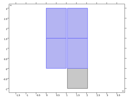
Click to expand the Layers section. In the table, enter the following settings:
The first rectangle consists of two rectangular domains representing the vacuum and metamaterial, respectively.
PML model
1
In the Geometry toolbar, click  Rectangle.
2
In the Settings window for Rectangle, type PML model in the Label text field.
3
Locate the Size and Shape section. In the Height text field, type 4.
4
Locate the Position section. In the x text field, type 1.05.
5
In the y text field, type -1.
6
Locate the Layers section. In the table, enter the following settings:
The second rectangle consists of three rectangular domains representing the vacuum, metamaterial, and PML.
7
Click  Build All Objects.
8
Click the  Zoom Extents button in the Graphics toolbar.
Electromagnetic Waves, Frequency Domain (ewfd)
Next, set up the physics. Use two different ways to model the infinite metamaterial domain.
1
In the Model Builder window, under Component 1 (comp1) click Electromagnetic Waves, Frequency Domain (ewfd).
2
In the Settings window for Electromagnetic Waves, Frequency Domain, locate the Components section.
3
From the Electric field components solved for list, choose Out-of-plane vector.
Wave Equation, Electric 1
1
In the Model Builder window, under Component 1 (comp1)>Electromagnetic Waves, Frequency Domain (ewfd) click Wave Equation, Electric 1.
2
In the Settings window for Wave Equation, Electric, locate the Electric Displacement Field section.
3
From the Electric displacement field model list, choose Relative permittivity.
Port 1
1
In the Physics toolbar, click  Boundaries and choose Port.
2
For the first port, wave excitation is on by default.
3
In the Settings window for Port, locate the Port Properties section.
4
From the Type of port list, choose Periodic.
5
Locate the Port Mode Settings section. Specify the E0 vector as
6
In the α text field, type alpha.
7
Locate the Automatic Diffraction Order Calculation section. In the n text field, type n_a.
Port 2
1
In the Physics toolbar, click  Boundaries and choose Port.
2
3
In the Settings window for Port, locate the Port Properties section.
4
From the Type of port list, choose Periodic.
5
Locate the Port Mode Settings section. Specify the E0 vector as
6
Locate the Automatic Diffraction Order Calculation section. In the n text field, type n_b.
The first method uses two ports.
Periodic Condition 1
1
In the Physics toolbar, click  Boundaries and choose Periodic Condition.
2
3
In the Settings window for Periodic Condition, locate the Periodicity Settings section.
4
From the Type of periodicity list, choose Floquet periodicity.
5
From the k-vector for Floquet periodicity list, choose From periodic port.
Port 3
1
In the Physics toolbar, click  Boundaries and choose Port.
2
3
In the Settings window for Port, locate the Port Properties section.
4
From the Wave excitation at this port list, choose On.
5
From the Type of port list, choose Periodic.
6
Locate the Port Mode Settings section. Specify the E0 vector as
7
In the α text field, type alpha.
8
Locate the Automatic Diffraction Order Calculation section. In the n text field, type n_a.
Periodic Condition 2
1
In the Physics toolbar, click  Boundaries and choose Periodic Condition.
2
3
In the Settings window for Periodic Condition, locate the Periodicity Settings section.
4
From the Type of periodicity list, choose Floquet periodicity.
5
From the k-vector for Floquet periodicity list, choose From periodic port.
Definitions
Perfectly Matched Layer 1 (pml1)
1
In the Definitions toolbar, click  Perfectly Matched Layer.
2
3
In the Settings window for Perfectly Matched Layer, locate the Scaling section.
4
In the PML scaling factor text field, type -1.
The second method uses one port and the PML.
Electromagnetic Waves, Frequency Domain (ewfd)
Transition Boundary Condition 1
1
In the Physics toolbar, click  Boundaries and choose Transition Boundary Condition.
2
3
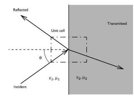
In the Settings window for Transition Boundary Condition, locate the Transition Boundary Condition section.
4
From the Electric displacement field model list, choose Relative permittivity.
5
From the μr list, choose User defined. In the associated text field, type mu_a.
6
From the εr list, choose User defined. In the associated text field, type e_a.
7
From the σ list, choose User defined. Leave the default value 0.
8
In the d text field, type lda0/1000.
Materials
Material 1 (mat1)
1
In the Model Builder window, under Component 1 (comp1) right-click Materials and choose Blank Material.
2
3
In the Settings window for Material, locate the Material Contents section.
4
Material 2 (mat2)
1
Right-click Materials and choose Blank Material.
2
3
In the Settings window for Material, locate the Material Contents section.
4
Study 1
Step 1: Frequency Domain
1
In the Model Builder window, under Study 1 click Step 1: Frequency Domain.
2
In the Settings window for Frequency Domain, locate the Study Settings section.
3
In the Frequencies text field, type f0.
Mesh 1
In the Model Builder window, under Component 1 (comp1) right-click Mesh 1 and choose Build All.
Study 1
In the Home toolbar, click  Compute.
Results
Study 1/Solution 1 (sol1)
The PML is not of interest for the result visualization; use only the air and metamaterial domains for this purpose.
1
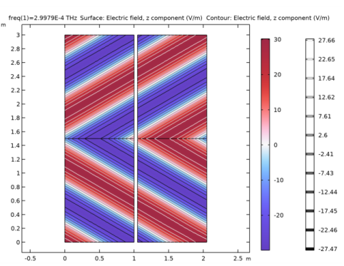
In the Model Builder window, expand the Results>Datasets node, then click Study 1/Solution 1 (sol1).
Selection
1
In the Results toolbar, click  Attributes and choose Selection.
2
In the Settings window for Selection, locate the Geometric Entity Selection section.
3
From the Geometric entity level list, choose Domain.
4
Electric Field (ewfd)
The default plot shows the norm of the electric field. Modify the plot to show the z component of the electric field, then add a contour plot.
Surface 1
1
In the Model Builder window, expand the Electric Field (ewfd) node, then click Surface 1.
2
In the Settings window for Surface, locate the Expression section.
3
In the Expression text field, type Ez.
4
Locate the Coloring and Style section. From the Color table list, choose WaveLight.
Contour 1
1
In the Model Builder window, right-click Electric Field (ewfd) and choose Contour.
2
In the Settings window for Contour, locate the Expression section.
3
In the Expression text field, type Ez.
4
Locate the Levels section. In the Total levels text field, type 12.
5
Locate the Coloring and Style section. From the Color table list, choose GrayPrint.
6
Click the  Zoom Extents button in the Graphics toolbar. Compare the resulting plot with that shown in Figure 2.