PDF

Two-Phase Flow in Column
Introduction
The following example analyzes two-phase flow in porous media. Describing how immiscible fluids move through porous media is key to answering many environmental and industrial questions. Unfortunately, multiphase analyses are complicated by the need to solve for multiple dependent variables along with a variety of unknowns. Among them are hydraulic properties that depend on the pressure and saturation levels of each fluid phase.
This problem demonstrates two-phase flow following a U.S. Environmental Protection Agency experimental setup (Ref. 1). This straightforward experiment matches observations for a laboratory column to numerical estimates of two-phase flow. With these column experiments, the researchers evaluated flow for varying fluid pairs (air-water, air-oil, and oil-water) and then match the experimental results to those from computer simulations that employ analytic expressions for retention and permeability. This discussion addresses their work for the Lincoln soil and use formulas from Mualem (Ref. 2) and van Genuchten (Ref. 3) to give hydraulic properties.
Figure 1: Geometry of the two-phase flow column experiments in Hopmans and others (Ref. 1).
This is a multipart example. The first part sets up the two-phase flow model for water and air; the equations solve for pressures. Saturation varies with the solution. An underlying assumption is that at least some residual air and water exist throughout the soil column at all times. The model tracks the gas front as it displaces a wetting fluid by observing saturation rather than assuming a discrete interface. The second part modifies the air-water simulation for air-oil and oil-water mixtures.
Model Definition
In the experimental setup for air and water, air enters from the top surface of a column made of water and sand. The incoming air (the nonwetting phase) forces the water (the wetting phase) toward the outlet at the base of the column. At the inlet, air pressure increases by steps in time, and no water exits through the column top. In moving to the outlet, the water passes through a disc that is impermeable to airflow. Neither the air nor the water can pass through the vertical column walls. The water pressure at the outlet, which changes in time, corresponds to the height of fluid rise in a receiving buret. The column has a total height of 8.34 cm, a 6-cm radius, and the disk is 0.74 cm thick. The experiment covers 170 hours.
Governing Equations and Boundary Conditions
Two-phase flow in porous media follows separate equations for the wetting (w) and nonwetting (nw) fluids:
(1)
(2)
where θs is the total porosity or saturated volume fraction; θr is the residual volume fraction, so the difference θs-θr is the available pore space for phases to move; Se is the effective saturation; t is time; κint is the intrinsic permeability of the porous medium (m2); kr is the relative permeability (a function of saturation for a given fluid); μ is the fluid’s dynamic viscosity (Pa·s); p is pressure (Pa); ρ is the fluid density (kg/m3); g is acceleration of gravity; and D is the coordinate (for example, x, y, or z) of vertical elevation (m).
When considering a continuous fluid field, neither phase ever completely fills the pore space, giving a volume fraction for the wetting phase, θw, and nonwetting phase, θnw. For the wetting phase, θ varies from zero or a small residual value θr to the total porosity, θs. The effective saturation, Se, comes from scaling θ with respect to θs and θr and so varies from 0 to 1. Both θ and Se are functions of the pressures of both fluids in the system.
The capillary pressure pc is commonly defined as the difference between the pressure of the nonwetting and wetting phases
(3)
The available pore space can be completely filled with one fluid at a given time, which relates the effective saturations for each phase
(4)
The specific capacity of the wetting phase depends on changes in the effective saturation with respect to the capillary pressure as
(5)
in the same way, the specific capacity of the nonwetting phase is defined with the help of Equation 4 as
Since the specific capacity of the two phases is the same but with opposite sign, it is just denoted as .
Using Equation 3, Equation 4, and Equation 5 in Equation 1 and Equation 2 simplifies the numerical model. The governing equations become:
You can solve this system of equations simultaneously for pw and pnw. In this example, the two fluids are incompressible, but that need not be the case. Rearranging terms, and adding the density of each fluid, we obtain two coupled Darcy’s law equations, one for the wetting phase, and another for the nonwetting phase
Initially, the water and air in the column follow hydrostatic distributions. The boundary conditions allow the water to exit only from the base of the soil column. For the wetting phase, the boundary conditions are
where n is the unit vector normal to the boundary.
Because air enters at the column top but never exits, the boundary conditions for the nonwetting phase are
Retention and Permeability Relationships
You can set up this two-phase flow analysis using interpolation from experimental data, arbitrary mathematical formulas, or results from other equations in the model to define how θ, C, Se, kr, and pc vary simultaneously. The existing model uses retention and permeability relationships from Ref. 2 and Ref. 3 that express changes in θ, C, Se, and kr as a function of the capillary pressure pc. Because pc is large and because changes in θ, C, Se, and kr are small, these expressions transform capillary pressure to the equivalent height of water or capillary pressure head as in Hc = pc/(ρwater g). The hydraulic properties relative to the wetting fluid in van Genuchten retention model are
where α, n, m, and L denote soil characteristics. Note that with two-phase flow, the van Genuchten-Mualem formulas hinge on the value of Hc.
For the nonwetting fluid, the properties
arise from the definitions for the wetting phase.
Different Fluid Pairs
When switching between air-water, air-oil, and oil-water experiments, the authors used different scaling with interfacial tensions according to Leverett (Ref. 4). The Leverett scaling adjusts the nonwetting phase pressure at the column top to produce the same volume of wetting fluid outflow at the column bottom regardless of the fluid pair. With Leverett scaling, switching between fluid pairs requires using the correct fluid properties ρ and μ for the fluid pair and adjusting the boundary and initial pressures according to
In these equations, σ represents the interfacial tension between the different fluids, and the subscripts denote the fluid pair. These values appear in a table at the end of this section. For example, σaoaw equals 0.373, and σowaw equals 0.534; further, the first nonwetting phase pressure head (in meters of water) is 0.4 m for the air-water system, 0.1 m for the air-oil system, and 0.2 m for the water-oil system.
Because relative permeability and retention properties for a porous medium depend on the fluid moving through it, switching fluid pairs also requires switching the retention and permeability properties in the model. This requirement can mean inserting new experimental data or adjusting mathematical formulas. In this model, the authors assessed the permeability and retention parameters were assessed by curve fitting to analytic formulas. They adjusted the parameters α, n, κs, and θr to get the best fit for each fluid. A review of the data tables that follow reveals that the ratios in the α values for the different fluid pairs roughly equals the σ ratios just given.
Implementation: Step Change on a Boundary
The following step-by-step instructions define the timing of the stepped nonwetting phase pressures at the inlet by using an interpolation function. Interpolating in COMSOL Multiphysics is straightforward. Add an Interpolation function under Global Definitions, set up the table with the times and corresponding pressure heads, assign a name to the interpolation function, and use it where the function is needed. To activate the functions created, simply enter the function name (for example, Hp_nw_t) along with the argument — that is, the time t in parentheses. For example, you define the nonwetting pressure as
p_nw = Hp_nw_t(t)*rho_water*g_const
The density of water appears in the equation because Ref. 1 defines the boundary pressure as a height of water.
Figure 2: Interpolation function used for Hp_nw_t(t).
Data
The data used in this model correspond to the air-water experiments for the Lincoln sand as reported in Ref. 1:
ρw
μw
1·10-3 Pa·s
ρa
μa
1.81·10-5 Pa·s
κint
κs
θs
θs,u
pnw,top
The van Genuchten parameters for the different fluid pairs are the following:
qr,w
α
m-1
κs
m-2
Pressure head at the air inlet increments in time according to the table below, see Figure 2.
At the water outlet, the fluid level in the receiving buret increases linearly in time from 0 m to 0.1 m.
Results and Discussion
Figure 3 shows an early-time snapshot from the COMSOL Multiphysics solution for two-phase flow in a laboratory column. The shading depicts the effective saturation of the nonwetting phase (air), while the arrows give the wetting phase (water) velocities.
Figure 3: Solution to two-phase flow model at 0.1 hours: nonwetting phase saturation (surface plot). Results correspond to air-water experiment on Lincoln soil from the US EPA.
The image illustrates the nonwetting fluid entering the soil column and displacing the wetting fluid. The nonwetting phase enters because it is being forced into the inlet with a multi-step pressure change.
Figure 4 shows the stepped pressure head used at the inlet boundary along with the capillary pressure in the column at various elevations. Specifying the point locations during postprocessing circumvents the need to plan observation sites during input. The solution to the two-phase flow problem provided is an excellent match to the results of Ref. 1.
That the capillary pressure head and the air inlet pressure in Figure 4 track together is what made the laboratory setup successful. To get high resolution on the permeability and retention behaviors, the authors in Ref. 1 set the pressure steps large enough that the impact is instantaneous in the soil column. As shown in Figure 5, the permeability changes instantaneously throughout the column.
Figure 4: Inlet air pressure head (solid line) and capillary pressure head (dashed lines) for air-water flow in Lincoln soil.
Figure 5: Relative permeability functions for water (solid lines) and air (dashed lines) for Lincoln soil at three different points.
Solutions for two-phase flow for the air-oil and oil-water systems appear in Figure 6 and Figure 7, respectively.
Figure 6: Inlet-air pressure head (solid line) and capillary pressure head (dashed lines) for air-oil flow in Lincoln soil.
Figure 7: Inlet-air pressure head (solid line) and capillary pressure head (dashed lines) for oil-water flow in Lincoln soil.
The COMSOL Multiphysics results for the air-oil and oil-water two-phase flow problems prove to be in agreement to the results shown in Ref. 1. Through Leverett scaling you set the inlet pressure so that the air-oil and oil-water systems would produce the volume outflow rate from the air-water experiment. As with the air-water system, the capillary pressure head and air-inlet pressure for the air-oil experiment track instantaneously. For the water-oil system, however, there is a lag between the nonwetting and wetting phase pressures.
References
1. J.W. Hopmans, M.E. Grismer, J. Chen, and Y.P. Liu, Parameter Estimation of Two-fluid Capillary Pressure Saturation and Permeability Functions, U.S. Environmental Protection Agency EPA/600/R-98/046, Cincinnati, Ohio, 1998.
2. Y. Mualem, “A new model for predicting the hydraulic permeability of unsaturated porous media”, Water Res. Research, vol. 12, pp. 513–522, 1976.
3. M.Th. van Genuchten, “A closed-form equation for predicting the hydraulic of conductivity of unsaturated soils”, Soil Sci. Soc. Am. J., vol. 44, pp. 892–898, 1980.
4. M.C. Leverett, “Capillary behavior in porous solids”, Trans. AIME, vol. 142, pp. 152–169, 1941.
Application Library path: Subsurface_Flow_Module/Fluid_Flow/twophase_flow_column
Modeling Instructions
From the File menu, choose New.
New
In the New window, click  Model Wizard.
Model Wizard
1
In the Model Wizard window, click  2D.
2
In the Select Physics tree, select Fluid Flow>Porous Media and Subsurface Flow>Darcy’s Law (dl).
3
Click Add.
4
In the Pressure text field, type p_w.
5
In the Select Physics tree, select Fluid Flow>Porous Media and Subsurface Flow>Darcy’s Law (dl).
6
Click Add.
7
In the Pressure text field, type p_nw.
8
Click  Study.
9
In the Select Study tree, select General Studies>Time Dependent.
10
Global Definitions
Parameters 1
1
In the Model Builder window, under Global Definitions click Parameters 1.
2
In the Settings window for Parameters, locate the Parameters section.
3
Click  Load from File.
4
Define an interpolation function for the stepped pressure on the non-wetting phase boundary using the data available in a file.
Inlet air pressure head
1
In the Home toolbar, click  Functions and choose Global>Interpolation.
2
In the Settings window for Interpolation, locate the Definition section.
3
From the Data source list, choose File.
4
Click  Browse.
5
6
Click  Import.
7
Locate the Units section. In the Function table, enter the following settings:
8
In the Argument table, enter the following settings:
9
Locate the Definition section. In the Function name text field, type Hp_nw_t.
10
In the Label text field, type Inlet air pressure head.
11
Click  Plot, and compare with Figure 2
Geometry 1
Rectangle 1 (r1)
1
In the Geometry toolbar, click  Rectangle.
2
In the Settings window for Rectangle, locate the Size and Shape section.
3
In the Height text field, type 0.0834.
4
In the Width text field, type 0.06.
5
Click to expand the Layers section. In the table, enter the following settings:
6
Click  Build All Objects.
Definitions
The following modeling steps create a step function that is used later to create a smooth ramp for the effective saturation.
Ramp 1 (rm1)
1
In the Home toolbar, click  Functions and choose Local>Ramp.
2
In the Settings window for Ramp, click to expand the Smoothing section.
3
Select the Size of transition zone at start check box.
4
Add variables to simulate two-phase flow for the air-water system.
Air-water experiment
1
In the Home toolbar, click  Variables and choose Local Variables.
2
In the Settings window for Variables, type Air-water experiment in the Label text field.
3
Locate the Variables section. Click  Load from File.
4
Import the variables that define the Van Genuchten retention model, initial and boundary conditions as well as the material properties of the lower and the upper layers. The parameters are presented in the Data section.
Van Genuchten retention model
1
In the Home toolbar, click  Variables and choose Local Variables.
2
In the Settings window for Variables, type Van Genuchten retention model in the Label text field.
3
Locate the Variables section. Click  Load from File.
4
Initial and boundary conditions
1
In the Home toolbar, click  Variables and choose Local Variables.
2
In the Settings window for Variables, type Initial and boundary conditions in the Label text field.
3
Locate the Variables section. Click  Load from File.
4
Lower layer
1
In the Home toolbar, click  Variables and choose Local Variables.
2
In the Settings window for Variables, type Lower layer in the Label text field.
3
Locate the Geometric Entity Selection section. From the Geometric entity level list, choose Domain.
4
5
Locate the Variables section. Click  Load from File.
6
Upper layer
1
In the Home toolbar, click  Variables and choose Local Variables.
2
In the Settings window for Variables, type Upper layer in the Label text field.
3
Locate the Geometric Entity Selection section. From the Geometric entity level list, choose Domain.
4
5
Locate the Variables section. Click  Load from File.
6
Darcy’s Law (dl)
1
In the Model Builder window, under Component 1 (comp1) click Darcy’s Law (dl).
2
In the Settings window for Darcy’s Law, locate the Gravity Effects section.
3
Select the Include gravity check box.
Fluid 1
1
In the Model Builder window, under Component 1 (comp1)>Darcy’s Law (dl)>Porous Medium 1 click Fluid 1.
2
In the Settings window for Fluid, locate the Fluid Properties section.
3
From the ρ list, choose User defined. In the associated text field, type rho_w.
4
From the μ list, choose User defined. In the associated text field, type mu_w.
Porous Matrix 1
1
In the Model Builder window, click Porous Matrix 1.
2
In the Settings window for Porous Matrix, locate the Matrix Properties section.
3
From the εp list, choose User defined. In the associated text field, type 0.25.
4
From the κ list, choose User defined. In the associated text field, type kap_s.
Porous Medium 2
1
In the Model Builder window, under Component 1 (comp1)>Darcy’s Law (dl) right-click Porous Medium 1 and choose Duplicate.
2
3
In the Settings window for Porous Medium, locate the Porous Medium section.
4
From the Storage model list, choose User defined. In the Sp text field, type Cp.
Porous Matrix 1
1
In the Model Builder window, expand the Porous Medium 2 node, then click Porous Matrix 1.
2
In the Settings window for Porous Matrix, locate the Matrix Properties section.
3
In the κ text field, type kap_s*kr_w.
Initial Values 1
1
In the Model Builder window, under Component 1 (comp1)>Darcy’s Law (dl) click Initial Values 1.
2
In the Settings window for Initial Values, locate the Initial Values section.
3
In the pw text field, type p_w_init.
Pressure 1
1
In the Physics toolbar, click  Boundaries and choose Pressure.
2
3
In the Settings window for Pressure, locate the Pressure section.
4
In the p0 text field, type p_w0.
Mass Source 1
1
In the Physics toolbar, click  Domains and choose Mass Source.
2
3
In the Settings window for Mass Source, locate the Mass Source section.
4
In the Qm text field, type Cp*p_nwt*rho_w.
Darcy’s Law 2 (dl2)
1
In the Model Builder window, under Component 1 (comp1) click Darcy’s Law 2 (dl2).
2
3
In the Settings window for Darcy’s Law, locate the Gravity Effects section.
4
Select the Include gravity check box.
Porous Medium 1
1
In the Model Builder window, under Component 1 (comp1)>Darcy’s Law 2 (dl2) click Porous Medium 1.
2
In the Settings window for Porous Medium, locate the Porous Medium section.
3
From the Storage model list, choose User defined. In the Sp text field, type Cp.
Fluid 1
1
In the Model Builder window, click Fluid 1.
2
In the Settings window for Fluid, locate the Fluid Properties section.
3
From the ρ list, choose User defined. In the associated text field, type rho_nw.
4
From the μ list, choose User defined. In the associated text field, type mu_nw.
Porous Matrix 1
1
In the Model Builder window, click Porous Matrix 1.
2
In the Settings window for Porous Matrix, locate the Matrix Properties section.
3
From the εp list, choose User defined. In the associated text field, type 0.25.
4
From the κ list, choose User defined. In the associated text field, type kap_s*kr_nw.
Initial Values 1
1
In the Model Builder window, under Component 1 (comp1)>Darcy’s Law 2 (dl2) click Initial Values 1.
2
In the Settings window for Initial Values, locate the Initial Values section.
3
In the pnw text field, type p_nw_init.
Pressure 1
1
In the Physics toolbar, click  Boundaries and choose Pressure.
2
3
In the Settings window for Pressure, locate the Pressure section.
4
In the p0 text field, type p_nw_top.
Mass Source 1
1
In the Physics toolbar, click  Domains and choose Mass Source.
2
3
In the Settings window for Mass Source, locate the Mass Source section.
4
In the Qm text field, type Cp*p_wt*rho_nw.
Mesh 1
Mapped 1
1
In the Mesh toolbar, click  Mapped.
2
In the Settings window for Mapped, locate the Domain Selection section.
3
From the Geometric entity level list, choose Entire geometry.
Size
1
In the Model Builder window, click Size.
2
In the Settings window for Size, locate the Element Size section.
3
From the Predefined list, choose Extra fine.
4
Click  Build All.
Air-water
1
In the Model Builder window, click Study 1.
2
In the Settings window for Study, type Air-water in the Label text field.
3
Locate the Study Settings section. Clear the Generate default plots check box.
Step 1: Time Dependent
1
In the Model Builder window, under Air-water click Step 1: Time Dependent.
2
In the Settings window for Time Dependent, locate the Study Settings section.
3
From the Time unit list, choose h.
4
In the Output times text field, type 0 0.001 0.01 0.1 range(1,170).
5
In the Home toolbar, click  Compute.
Results
Create point datasets for plotting the capillary pressure head and the relative permeabilities at several points.
Cut Point 2D 1
1
In the Model Builder window, expand the Results node.
2
Right-click Results>Datasets and choose Cut Point 2D.
3
In the Settings window for Cut Point 2D, locate the Point Data section.
4
In the X text field, type 0 0 0.
5
In the Y text field, type 0.075 0.045 0.015.
6
Next, reproduce the plot in Figure 4.
Inlet air pressure and capillary pressure, air-water
1
In the Results toolbar, click  1D Plot Group.
2
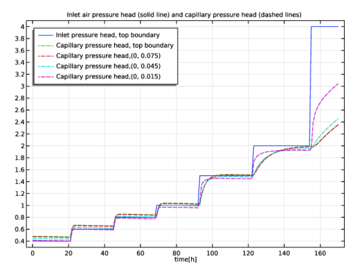
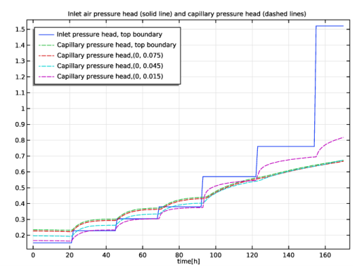
In the Settings window for 1D Plot Group, type Inlet air pressure and capillary pressure, air-water in the Label text field.
3
Locate the Plot Settings section. Select the x-axis label check box.
4
5
Click to expand the Title section. From the Title type list, choose Manual.
6
In the Title text area, type Inlet air pressure head (solid line) and capillary pressure head (dashed lines).
7
Locate the Legend section. From the Position list, choose Upper left.
Point Graph 1
1
Right-click Inlet air pressure and capillary pressure, air-water and choose Point Graph.
2
3
In the Settings window for Point Graph, locate the y-Axis Data section.
4
In the Expression text field, type Hp_nw_t(t).
5
Click to expand the Legends section. Select the Show legends check box.
6
From the Legends list, choose Manual.
7
8
In the Inlet air pressure and capillary pressure, air-water toolbar, click  Plot.
Point Graph 2
1
Right-click Point Graph 1 and choose Duplicate.
2
In the Settings window for Point Graph, click Replace Expression in the upper-right corner of the y-Axis Data section. From the menu, choose Component 1 (comp1)>Definitions>Variables>Hc - Capillary pressure head - m.
3
Click to expand the Coloring and Style section. Find the Line style subsection. From the Line list, choose Dashed.
4
Locate the Legends section. From the Legends list, choose Automatic.
5
Find the Include subsection. Clear the Point check box.
6
Select the Description check box.
7
Find the Prefix and suffix subsection. In the Suffix text field, type , top boundary.
8
In the Inlet air pressure and capillary pressure, air-water toolbar, click  Plot.
Point Graph 3
1
Right-click Point Graph 2 and choose Duplicate.
2
In the Settings window for Point Graph, locate the Data section.
3
From the Dataset list, choose Cut Point 2D 1.
4
Locate the Legends section. Find the Include subsection. Select the Point check box.
5
Clear the Description check box.
6
Find the Prefix and suffix subsection. Clear the Suffix text field.
7
In the Prefix text field, type Capillary pressure head, .
8
In the Inlet air pressure and capillary pressure, air-water toolbar, click  Plot.
To generate the plots in Figure 5 and Figure 3, continue with the steps below.
Relative permeabilities at 3 points
1
In the Home toolbar, click  Add Plot Group and choose 1D Plot Group.
2
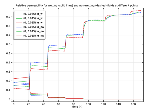
In the Settings window for 1D Plot Group, type Relative permeabilities at 3 points in the Label text field.
3
Locate the Data section. From the Dataset list, choose Cut Point 2D 1.
4
Locate the Title section. From the Title type list, choose Manual.
5
In the Title text area, type Relative permeability for wetting (solid lines) and non-wetting (dashed) fluids at different points.
6
Locate the Plot Settings section. Select the x-axis label check box.
7
8
Locate the Legend section. From the Position list, choose Upper left.
Point Graph 1
1
Right-click Relative permeabilities at 3 points and choose Point Graph.
2
In the Settings window for Point Graph, click Replace Expression in the upper-right corner of the y-Axis Data section. From the menu, choose Component 1 (comp1)>Definitions>Variables>kr_w - Relative permeability, wetting phase.
3
Locate the Legends section. Select the Show legends check box.
4
Find the Include subsection. Select the Expression check box.
5
In the Relative permeabilities at 3 points toolbar, click  Plot.
Point Graph 2
1
Right-click Point Graph 1 and choose Duplicate.
2
In the Settings window for Point Graph, click Replace Expression in the upper-right corner of the y-Axis Data section. From the menu, choose Component 1 (comp1)>Definitions>Variables>kr_nw - Relative permeability, non-wetting phase.
3
Locate the Coloring and Style section. Find the Line style subsection. From the Line list, choose Dashed.
4
From the Color list, choose Cycle (reset).
5
In the Relative permeabilities at 3 points toolbar, click  Plot.
2D Plot Group 3
1
In the Home toolbar, click  Add Plot Group and choose 2D Plot Group.
2
In the Settings window for 2D Plot Group, locate the Data section.
3
From the Time (h) list, choose 0.1.
Surface 1
1
Right-click 2D Plot Group 3 and choose Surface.
2
In the Settings window for Surface, click Replace Expression in the upper-right corner of the Expression section. From the menu, choose Component 1 (comp1)>Definitions>Variables>Se_nw - Effective saturation, non-wetting phase.
3
In the 2D Plot Group 3 toolbar, click  Plot.
4
Click the  Zoom Extents button in the Graphics toolbar.
Effective Saturation, non-wetting phase
1
In the Model Builder window, under Results click 2D Plot Group 3.
2
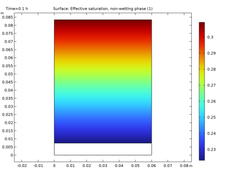
In the Settings window for 2D Plot Group, type Effective Saturation, non-wetting phase in the Label text field.
Perform similar studies with air-oil and oil-water to generate the plots in Figure 6 and Figure 7.
Definitions
Air-oil experiment
1
In the Home toolbar, click  Variables and choose Local Variables.
2
In the Settings window for Variables, type Air-oil experiment in the Label text field.
3
Locate the Variables section. Click  Load from File.
4
Oil-water experiment
1
In the Home toolbar, click  Variables and choose Local Variables.
2
In the Settings window for Variables, type Oil-water experiment in the Label text field.
3
Locate the Variables section. Click  Load from File.
4
Air-water
Step 1: Time Dependent
1
In the Model Builder window, under Air-water click Step 1: Time Dependent.
2
In the Settings window for Time Dependent, locate the Physics and Variables Selection section.
3
Select the Modify model configuration for study step check box.
4
In the tree, select Component 1 (Comp1)>Definitions>Air-Oil Experiment and Component 1 (Comp1)>Definitions>Oil-Water Experiment.
5
Add Study
1
In the Home toolbar, click  Add Study to open the Add Study window.
2
Go to the Add Study window.
3
Find the Studies subsection. In the Select Study tree, select General Studies>Time Dependent.
4
Click Add Study in the window toolbar.
5
In the Home toolbar, click  Add Study to close the Add Study window.
Air-oil
1
In the Model Builder window, click Study 2.
2
In the Settings window for Study, type Air-oil in the Label text field.
3
Locate the Study Settings section. Clear the Generate default plots check box.
Step 1: Time Dependent
1
In the Model Builder window, under Air-oil click Step 1: Time Dependent.
2
In the Settings window for Time Dependent, locate the Study Settings section.
3
From the Time unit list, choose h.
4
In the Output times text field, type 0 0.001 0.01 0.1 range(1,170).
5
Locate the Physics and Variables Selection section. Select the Modify model configuration for study step check box.
6
In the tree, select Component 1 (Comp1)>Definitions>Air-Water Experiment and Component 1 (Comp1)>Definitions>Oil-Water Experiment.
7
8
In the Home toolbar, click  Compute.
Results
Cut Point 2D 2
1
In the Model Builder window, under Results>Datasets right-click Cut Point 2D 1 and choose Duplicate.
2
In the Settings window for Cut Point 2D, locate the Data section.
3
From the Dataset list, choose Air-oil/Solution 2 (sol2).
Inlet air pressure and capillary pressure, air-oil
1
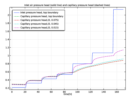
In the Model Builder window, right-click Inlet air pressure and capillary pressure, air-water and choose Duplicate.
2
In the Settings window for 1D Plot Group, type Inlet air pressure and capillary pressure, air-oil in the Label text field.
3
Locate the Data section. From the Dataset list, choose Air-oil/Solution 2 (sol2).
Point Graph 1
1
In the Model Builder window, expand the Inlet air pressure and capillary pressure, air-oil node, then click Point Graph 1.
2
In the Settings window for Point Graph, locate the y-Axis Data section.
3
In the Expression text field, type Hp_nw_t(t)*sigma.
Point Graph 3
1
In the Model Builder window, click Point Graph 3.
2
In the Settings window for Point Graph, locate the Data section.
3
From the Dataset list, choose Cut Point 2D 2.
4
In the Inlet air pressure and capillary pressure, air-oil toolbar, click  Plot.
Add Study
1
In the Home toolbar, click  Add Study to open the Add Study window.
2
Go to the Add Study window.
3
Find the Studies subsection. In the Select Study tree, select General Studies>Time Dependent.
4
Click Add Study in the window toolbar.
5
In the Home toolbar, click  Add Study to close the Add Study window.
Oil-water
1
In the Model Builder window, click Study 3.
2
In the Settings window for Study, type Oil-water in the Label text field.
3
Locate the Study Settings section. Clear the Generate default plots check box.
Step 1: Time Dependent
1
In the Model Builder window, under Oil-water click Step 1: Time Dependent.
2
In the Settings window for Time Dependent, locate the Study Settings section.
3
From the Time unit list, choose h.
4
In the Output times text field, type 0 0.001 0.01 0.1 range(1,170).
5
Locate the Physics and Variables Selection section. Select the Modify model configuration for study step check box.
6
In the tree, select Component 1 (Comp1)>Definitions>Air-Water Experiment and Component 1 (Comp1)>Definitions>Air-Oil Experiment.
7
8
In the Home toolbar, click  Compute.
Results
Cut Point 2D 3
1
In the Model Builder window, under Results>Datasets right-click Cut Point 2D 2 and choose Duplicate.
2
In the Settings window for Cut Point 2D, locate the Data section.
3
From the Dataset list, choose Oil-water/Solution 3 (sol3).
Inlet air pressure and capillary pressure, oil-water
1
In the Model Builder window, right-click Inlet air pressure and capillary pressure, air-oil and choose Duplicate.
2
In the Settings window for 1D Plot Group, type Inlet air pressure and capillary pressure, oil-water in the Label text field.
3
Locate the Data section. From the Dataset list, choose Oil-water/Solution 3 (sol3).
Point Graph 3
1
In the Model Builder window, expand the Inlet air pressure and capillary pressure, oil-water node, then click Point Graph 3.
2
In the Settings window for Point Graph, locate the Data section.
3
From the Dataset list, choose Cut Point 2D 3.
4
In the Inlet air pressure and capillary pressure, oil-water toolbar, click  Plot.