PDF

Solute Transport in Prescribed Groundwater Flow
Introduction
This model tracks a solute in a prescribed groundwater flow over 1000 days accounting for longitudinal and transversal dispersivity.
This set up is often used as a benchmark case to verify different implementations for modeling species transport. It compares the results with an analytical solution (Ref. 1).
Model Definition
The model geometry is a square with a side length of 4 km. Because the groundwater flow is prescribed, the model solves for species transport only with a predefined flow field of magnitude m/d.
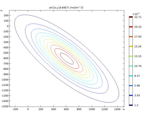
An initial concentration following a Gaussian distribution is applied. The analytical solution can be defined as a function in COMSOL. See Ref. 1 for the analytical expression. Because this expression is quite long and just used to compare the simulation results against it, a preset file is loaded that contains the analytical solution already (Figure 1).
Figure 1: Analytical solution for the concentration after 1000 days.
Results and Discussion
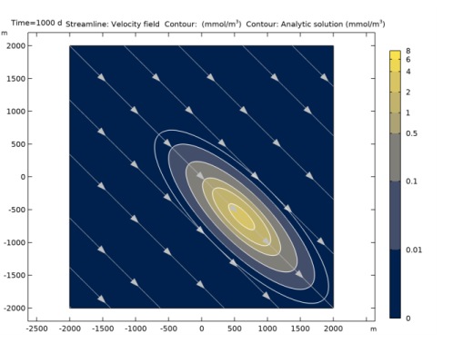
Figure 2 shows the result after 1000 days. The predefined flow field is visualized by an arrow streamline plot. The analytical solution is also plotted (white contour lines) and it can be seen that the simulation results (filled contours) matche the analytical solution.
Figure 2: Resulting concentration distribution after 1000 days (filled contours) compared with the analytical solution (white contours). Arrow streamlines visualize the prescribed flow direction.
Reference
1. J.L. Wilson and P.J. Miller, “Two-dimensional plume in uniform ground-water flow,” Journal of the Hydraulics Division, ASCE, 1978.
Application Library path: Subsurface_Flow_Module/Solute_Transport/solute_transport
Modeling Instructions
Application Libraries
1
From the File menu, choose Application Libraries.
2
In the Application Libraries window, select Subsurface Flow Module>Solute Transport>solute_transport_preset in the tree.
3
Add Component
In the Home toolbar, click  Add Component and choose 2D.
Geometry 1
Square 1 (sq1)
1
In the Geometry toolbar, click  Square.
2
In the Settings window for Square, locate the Size section.
3
In the Side length text field, type L.
4
Locate the Position section. From the Base list, choose Center.
5
Click  Build All Objects.
Add Physics
1
In the Home toolbar, click  Add Physics to open the Add Physics window.
2
Go to the Add Physics window.
3
In the tree, select Chemical Species Transport>Transport of Diluted Species in Porous Media (tds).
4
Click Add to Component 1 in the window toolbar.
5
In the Home toolbar, click  Add Physics to close the Add Physics window.
Transport of Diluted Species in Porous Media (tds)
Fluid 1
1
In the Model Builder window, under Component 1 (comp1)>Transport of Diluted Species in Porous Media (tds)>Porous Medium 1 click Fluid 1.
2
In the Settings window for Fluid, locate the Convection section.
3
Specify the u vector as
Porous Matrix 1
1
In the Model Builder window, click Porous Matrix 1.
2
In the Settings window for Porous Matrix, locate the Matrix Properties section.
3
From the εp list, choose User defined. In the associated text field, type ne.
Porous Medium 1
In the Model Builder window, click Porous Medium 1.
Dispersion 1
1
In the Physics toolbar, click  Attributes and choose Dispersion.
2
In the Settings window for Dispersion, locate the Dispersion section.
3
From the Dispersion tensor list, choose Dispersivity.
4
In the αL text field, type aL.
5
In the αT text field, type aT.
Inflow 1
1
In the Physics toolbar, click  Boundaries and choose Inflow.
2
Outflow 1
1
In the Physics toolbar, click  Boundaries and choose Outflow.
2
The source term is defined as initial value. First, define the 2D Gauss distribution as a function.
Definitions
Analytic 2 (an2)
1
In the Home toolbar, click  Functions and choose Global>Analytic.
2
In the Settings window for Analytic, type gaussian in the Function name text field.
3
Locate the Definition section. In the Expression text field, type 1/(2*pi*esrc^2)*exp(-(x^2+y^2)/(2*esrc^2)).
4
In the Arguments text field, type x, y.
5
Locate the Units section. In the table, enter the following settings:
6
In the Function text field, type 1.
7
Locate the Plot Parameters section. In the table, enter the following settings:
8
Transport of Diluted Species in Porous Media (tds)
Initial Values 1
1
In the Model Builder window, under Component 1 (comp1)>Transport of Diluted Species in Porous Media (tds) click Initial Values 1.
2
In the Settings window for Initial Values, locate the Initial Values section.
3
In the c text field, type M*gaussian(x-x0,y-y0).
Define a variable for the analytical solution which makes it easier to compare the results in postprocessing.
Definitions
Variables 1
1
In the Model Builder window, under Component 1 (comp1) right-click Definitions and choose Variables.
2
In the Settings window for Variables, locate the Variables section.
3
To resolve the spatial distribution, a fine mesh is required. Use a mapped mesh.
Mesh 1
Mapped 1
In the Mesh toolbar, click  Mapped.
Size
1
In the Model Builder window, click Size.
2
In the Settings window for Size, click to expand the Element Size Parameters section.
3
In the Maximum element size text field, type 20.
4
Click  Build All.
Add a time-dependent study to run the simulation over 1000 days. Restrict the maximum time step, for an accurate solution.
Add Study
1
In the Home toolbar, click  Add Study to open the Add Study window.
2
Go to the Add Study window.
3
Find the Studies subsection. In the Select Study tree, select General Studies>Time Dependent.
4
Click Add Study in the window toolbar.
5
In the Home toolbar, click  Add Study to close the Add Study window.
Study 1
Step 1: Time Dependent
1
In the Settings window for Time Dependent, locate the Study Settings section.
2
From the Time unit list, choose d.
3
In the Output times text field, type range(0,100,1000).
Solution 1 (sol1)
1
In the Study toolbar, click  Show Default Solver.
2
In the Model Builder window, expand the Solution 1 (sol1) node, then click Time-Dependent Solver 1.
3
In the Settings window for Time-Dependent Solver, click to expand the Time Stepping section.
4
From the Maximum step constraint list, choose Constant.
5
In the Maximum step text field, type 20.
6
Click  Compute.
Results
Concentration (tds)
To create Figure 2 proceed as follows.
Concentration compared
1
In the Home toolbar, click  Add Plot Group and choose 2D Plot Group.
2
In the Settings window for 2D Plot Group, type Concentration compared in the Label text field.
Streamline 1
1
Right-click Concentration compared and choose Streamline.
2
In the Settings window for Streamline, click Replace Expression in the upper-right corner of the Expression section. From the menu, choose Component 1 (comp1)>Transport of Diluted Species in Porous Media>tds.u,tds.v - Velocity field.
3
Locate the Streamline Positioning section. From the Positioning list, choose Uniform density.
4
In the Separating distance text field, type 0.1.
5
Locate the Coloring and Style section. Find the Point style subsection. From the Color list, choose Gray.
6
From the Type list, choose Arrow.
Contour 1
1
In the Model Builder window, right-click Concentration compared and choose Contour.
2
In the Settings window for Contour, locate the Expression section.
3
In the Unit field, type mmol/m^3.
4
Locate the Levels section. From the Entry method list, choose Levels.
5
In the Levels text field, type 0.001 0.01 0.1 0.5 1 2 4 6 8.
6
Locate the Coloring and Style section. From the Contour type list, choose Filled.
7
From the Color table list, choose Cividis.
8
From the Scale list, choose Logarithmic.
Contour 2
1
Right-click Concentration compared and choose Contour.
2
In the Settings window for Contour, click Replace Expression in the upper-right corner of the Expression section. From the menu, choose Component 1 (comp1)>Definitions>Variables>c_analytic - Analytic solution - mol/m³.
3
Locate the Expression section. In the Unit field, type mmol/m^3.
4
Locate the Levels section. From the Entry method list, choose Levels.
5
In the Levels text field, type 0.001 0.01 0.1 0.5 1 2 4 6 8.
6
Locate the Coloring and Style section. From the Coloring list, choose Uniform.
7
From the Color list, choose White.
8
Clear the Color legend check box.
9
In the Concentration compared toolbar, click  Plot. Compare with Figure 2.