PDF

Viscoelastic Structural Damper
Introduction
The example studies a forced response of a typical viscoelastic damper. Damping elements involving layers of viscoelastic materials are often used for reduction of seismic and wind induced vibrations in buildings and other tall structures. The common feature is that the frequency of the forced vibrations is low.
Model Definition
The geometry of the viscoelastic damper is shown in Figure 1 (from Ref. 1). The damper consists of two layers of viscoelastic material confined between mounting elements made of steel.
Figure 1: Viscoelastic damping element.
The viscoelastic layers are modeled with the generalized Maxwell model available in COMSOL Multiphysics. The generalized Maxwell model represents the viscoelastic material as a series of branches, each with a spring-dashpot pair.
Eighteen viscoelastic branches guarantee accurate representation of the material behavior for a wide range of excitation frequencies, when the damper is subjected to forced vibration. The values of the shear moduli and relaxation times for each branch are available in Ref. 1. They are summarized in the following table:
ρ
G1
τ1
10-7 s
G2
τ2
10-6 s
G3
τ3
G4
τ4
10-5 s
G5
τ5
G6
τ6
10-4 s
G7
τ7
G8
τ8
10-3 s
G9
τ9
G10
τ10
10-2 s
G11
τ11
G12
τ12
G13
τ13
G14
τ14
G15
8.25·10-2 MPa
τ15
G16
τ16
G17
3.73·10-2 MPa
τ17
G18
1.18·10-2 MPa
τ18
One of the mounting elements is fixed; the other two are loaded with periodic forces with frequencies in the range 05 Hz.
The time-domain representation of the forced solution is computed using the fast Fourier transform (FFT).
Results and Discussion
The harmonic response at 3 Hz is shown in Figure 2.
In the frequency domain, the viscoelastic properties of the material appear as the storage modulus and loss modulus. The computed variation of the viscoelastic moduli with frequency is shown in Figure 3. The result is in very good agreement with the experimental data (Figure 7 in Ref. 2)
.
Figure 2: Vertical displacement of the damper, harmonic response.
Figure 3: Viscoelastic storage modulus (solid line) and loss modulus (dashed line). Both quantities are normalized by 6.895 to simplify the comparison with Ref. 2.
The time domain solution obtained from a FFT for the case of an excitation frequency of 3 Hz is shown in Figure 4.
Figure 4: Displacement of the damper after 1/3 second of forced vibrations.
Finally, the total vertical force versus vertical displacement for one of the mounting holes is shown in Figure 5.
Figure 5: Hysteresis loop for an excitation frequency of 3 Hz over the time interval of 1/3 s.
Notes About the COMSOL Implementation
You model in 3D and use the Solid Mechanics interface with Linear Elastic Material, add the Viscoelasticity node to the domains representing the viscoelastic layers.
References
1. S.W. Park “Analytical Modeling of Viscoelastic Dampers for Structural and Vibration Control,” Int. J. Solids and Structures, vol. 38, pp. 694–701, 2001.
2. K.L. Shen and T.T. Soong, “Modeling of Viscoelastic Dampers for Structural Applications,” J. Eng. Mech., vol. 121, pp. 694–701, 1995.
Application Library path: Structural_Mechanics_Module/Dynamics_and_Vibration/viscoelastic_damper_frequency
Modeling Instructions
From the File menu, choose New.
New
In the New window, click  Model Wizard.
Model Wizard
1
In the Model Wizard window, click  3D.
2
In the Select Physics tree, select Structural Mechanics>Solid Mechanics (solid).
3
Click Add.
4
Click  Study.
5
In the Select Study tree, select General Studies>Frequency Domain.
6
Geometry 1
Import the predefined geometry from a file.
1
In the Geometry toolbar, click Insert Sequence and choose Insert Sequence.
2
The imported geometry should look similar to that shown in Figure 1.
Solid Mechanics (solid)
Linear Elastic Material 2
1
In the Model Builder window, under Component 1 (comp1) right-click Solid Mechanics (solid) and choose Material Models>Linear Elastic Material.
2
In the Settings window for Linear Elastic Material, locate the Linear Elastic Material section.
3
From the Specify list, choose Bulk modulus and shear modulus.
4
From the Use mixed formulation list, choose Pressure formulation.
5
Viscoelasticity 1
1
In the Physics toolbar, click  Attributes and choose Viscoelasticity.
Since there are 18 branches in this material model, the data has been collected in a text file which you can load.
2
In the Settings window for Viscoelasticity, locate the Viscoelasticity Model section.
3
4
Click  Delete.
5
Click  Load from File.
6
Add Material
1
In the Home toolbar, click  Add Material to open the Add Material window.
2
Go to the Add Material window.
3
In the tree, select Built-in>Steel AISI 4340.
4
Click Add to Component in the window toolbar.
Materials
Viscoelastic
1
In the Model Builder window, under Component 1 (comp1) right-click Materials and choose Blank Material.
2
In the Settings window for Material, type Viscoelastic in the Label text field.
3
4
Locate the Material Contents section. In the table, enter the following settings:
5
In the Home toolbar, click  Add Material to close the Add Material window.
6
In the Settings window for Materials, in the Graphics window toolbar, clicknext to  Colors, then choose Show Material Color and Texture.
Solid Mechanics (solid)
Fixed Constraint 1
1
In the Physics toolbar, click  Boundaries and choose Fixed Constraint.
2
In the Settings window for Fixed Constraint, locate the Boundary Selection section.
3
From the Selection list, choose Bottom Holes.
Prescribed Displacement 1
1
In the Physics toolbar, click  Boundaries and choose Prescribed Displacement.
2
In the Settings window for Prescribed Displacement, locate the Boundary Selection section.
3
From the Selection list, choose Right Hole.
4
Locate the Prescribed Displacement section. Select the Prescribed in x direction check box.
5
Select the Prescribed in y direction check box.
Boundary Load 1
1
In the Physics toolbar, click  Boundaries and choose Boundary Load.
2
In the Settings window for Boundary Load, locate the Boundary Selection section.
3
From the Selection list, choose Right Hole.
4
Locate the Force section. Specify the FA vector as
Phase 1
1
In the Physics toolbar, click  Attributes and choose Phase.
2
In the Settings window for Phase, locate the Phase section.
3
Specify the φ vector as
Prescribed Displacement 2
1
In the Physics toolbar, click  Boundaries and choose Prescribed Displacement.
2
In the Settings window for Prescribed Displacement, locate the Boundary Selection section.
3
From the Selection list, choose Left Hole.
4
Locate the Prescribed Displacement section. Select the Prescribed in y direction check box.
Boundary Load 2
1
In the Physics toolbar, click  Boundaries and choose Boundary Load.
2
In the Settings window for Boundary Load, locate the Boundary Selection section.
3
From the Selection list, choose Left Hole.
4
Locate the Force section. Specify the FA vector as
Mesh 1
Free Quad 1
1
In the Mesh toolbar, click  Boundary and choose Free Quad.
2
Size 1
1
Right-click Free Quad 1 and choose Size.
2
In the Settings window for Size, locate the Element Size section.
3
From the Predefined list, choose Finer.
Distribution 1
1
In the Model Builder window, right-click Free Quad 1 and choose Distribution.
2
Swept 1
1
In the Mesh toolbar, click  Swept.
2
In the Settings window for Swept, locate the Domain Selection section.
3
From the Geometric entity level list, choose Domain.
4
Distribution 1
1
Right-click Swept 1 and choose Distribution.
2
In the Settings window for Distribution, locate the Distribution section.
3
In the Number of elements text field, type 2.
Free Quad 2
1
In the Mesh toolbar, click  Boundary and choose Free Quad.
2
Size 1
1
Right-click Free Quad 2 and choose Size.
2
In the Settings window for Size, locate the Element Size section.
3
From the Predefined list, choose Fine.
Swept 2
1
In the Mesh toolbar, click  Swept.
2
In the Settings window for Swept, locate the Domain Selection section.
3
From the Geometric entity level list, choose Domain.
4
Distribution 1
1
Right-click Swept 2 and choose Distribution.
2
In the Settings window for Distribution, locate the Distribution section.
3
In the Number of elements text field, type 2.
Copy Domain 1
1
In the Model Builder window, right-click Mesh 1 and choose Copying Operations>Copy Domain.
2
3
In the Settings window for Copy Domain, locate the Destination Domains section.
4
Click to select the  Activate Selection toggle button.
5
Free Quad 3
1
In the Mesh toolbar, click  Boundary and choose Free Quad.
2
Swept 3
1
In the Mesh toolbar, click  Swept.
2
In the Settings window for Swept, click  Build All.
The complete mesh should look similar to that shown in the figure below.
Study 1
Step 1: Frequency Domain
1
In the Model Builder window, under Study 1 click Step 1: Frequency Domain.
2
In the Settings window for Frequency Domain, locate the Study Settings section.
3
In the Frequencies text field, type range(0,0.125,0.5) range(1,0.5,5).
Solution 1 (sol1)
In the Study toolbar, click  Show Default Solver.
Results
Before computing the solution, set up a displacement plot that will be displayed and updated after every frequency response computation.
Displacement, Frequency Domain
1
In the Home toolbar, click  Add Plot Group and choose 3D Plot Group.
2
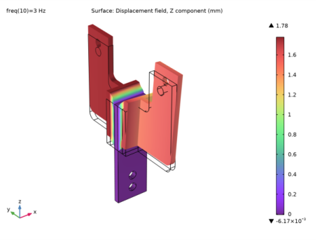
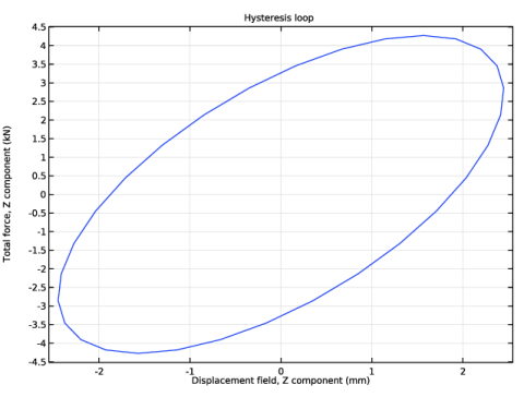
In the Settings window for 3D Plot Group, type Displacement, Frequency Domain in the Label text field.
Surface 1
1
Right-click Displacement, Frequency Domain and choose Surface.
2
In the Settings window for Surface, click Replace Expression in the upper-right corner of the Expression section. From the menu, choose Component 1 (comp1)>Solid Mechanics>Displacement>Displacement field - m>w - Displacement field, Z component.
3
Locate the Expression section. From the Unit list, choose mm.
4
Locate the Coloring and Style section. From the Color table list, choose SpectrumLight.
Deformation 1
Right-click Surface 1 and choose Deformation.
Study 1
Step 1: Frequency Domain
1
In the Settings window for Frequency Domain, click to expand the Results While Solving section.
2
Select the Plot check box.
Solution 1 (sol1)
In the Model Builder window, under Study 1>Solver Configurations right-click Solution 1 (sol1) and choose Compute.
Results
Displacement, Frequency Domain
1
In the Settings window for 3D Plot Group, locate the Data section.
2
From the Parameter value (freq (Hz)) list, choose 3.
3
Locate the Color Legend section. Select the Show maximum and minimum values check box.
4
In the Displacement, Frequency Domain toolbar, click  Plot.
The computed solution should closely resemble that shown in Figure 2.
To plot the storage and loss moduli, follow these steps:
Cut Point 3D 1
1
In the Results toolbar, click  Cut Point 3D.
2
In the Settings window for Cut Point 3D, locate the Point Data section.
3
In the X text field, type 0.
4
In the Z text field, type 0.
5
In the Y text field, type -10.
Storage and Loss Moduli
1
In the Results toolbar, click  1D Plot Group.
2
In the Settings window for 1D Plot Group, type Storage and Loss Moduli in the Label text field.
3
Locate the Data section. From the Dataset list, choose Cut Point 3D 1.
4
Click to expand the Title section. From the Title type list, choose Manual.
5
In the Title text area, type Storage and loss moduli.
6
Locate the Legend section. From the Position list, choose Upper left.
Point Graph 1
1
Right-click Storage and Loss Moduli and choose Point Graph.
2
In the Settings window for Point Graph, locate the y-Axis Data section.
3
In the Expression text field, type solid.Gstor/6.895.
4
Click to expand the Coloring and Style section. In the Width text field, type 2.
5
Click to expand the Legends section. Select the Show legends check box.
6
From the Legends list, choose Manual.
7
Point Graph 2
1
In the Model Builder window, right-click Storage and Loss Moduli and choose Point Graph.
2
In the Settings window for Point Graph, locate the y-Axis Data section.
3
In the Expression text field, type solid.Gloss/6.895.
4
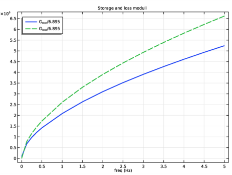
Click to expand the Coloring and Style section. Find the Line style subsection. From the Line list, choose Dashed.
5
In the Width text field, type 2.
6
Locate the Legends section. Select the Show legends check box.
7
From the Legends list, choose Manual.
8
9
In the Storage and Loss Moduli toolbar, click  Plot.
Add a new study to compute by using FFT the solution representation in time domain for the exitation frequency of 3 Hz.
Add Study
1
In the Home toolbar, click  Add Study to open the Add Study window.
2
Go to the Add Study window.
3
Find the Studies subsection. In the Select Study tree, select Empty Study.
4
5
In the Home toolbar, click  Add Study to close the Add Study window.
Study 2
Frequency to Time FFT
1
In the Study toolbar, click  Study Steps and choose Time Dependent>Frequency to Time FFT.
2
In the Settings window for Frequency to Time FFT, locate the Study Settings section.
3
From the Input study list, choose Study 1, Frequency Domain.
4
In the Times text field, type range(0,1/(3*30), 1/3).
5
Select the Use window function check box.
6
From the Window function list, choose Rectangular.
7
In the Window start text field, type 2.9.
8
In the Window end text field, type 3.1.
9
From the Scaling list, choose Discrete Fourier transform.
Definitions
Set up a variable to compute the time domain equivalent of the total force applied to one of the mounting holes.
Variables 1
1
In the Home toolbar, click  Variables and choose Local Variables.
2
In the Settings window for Variables, locate the Variables section.
3
4
In the Home toolbar, click  Compute.
Results
Displacement, Time Domain
The default plot will show the stress at the last time moment. Change it to visualize the vertical displacement as shown in Figure 4.
1
In the Settings window for 3D Plot Group, type Displacement, Time Domain in the Label text field.
2
Locate the Color Legend section. Select the Show maximum and minimum values check box.
Volume 1
1
In the Model Builder window, expand the Displacement, Time Domain node, then click Volume 1.
2
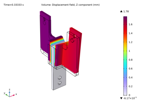
In the Settings window for Volume, click Replace Expression in the upper-right corner of the Expression section. From the menu, choose Component 1 (comp1)>Solid Mechanics>Displacement>Displacement field - m>w - Displacement field, Z component.
3
Locate the Expression section. From the Unit list, choose mm.
4
In the Displacement, Time Domain toolbar, click  Plot.
Hysteresis Loop
1
In the Home toolbar, click  Add Plot Group and choose 1D Plot Group.
Plot the total vertical force versus vertical displacement for one of the mounting holes, Figure 5.
2
In the Settings window for 1D Plot Group, type Hysteresis Loop in the Label text field.
3
Locate the Data section. From the Dataset list, choose Study 2/Solution 2 (sol2).
Point Graph 1
1
Right-click Hysteresis Loop and choose Point Graph.
2
In the Settings window for Point Graph, locate the Selection section.
3
Click to select the  Activate Selection toggle button.
4
5
Locate the y-Axis Data section. In the Expression text field, type Fz1.
6
From the Unit list, choose kN.
7
Locate the x-Axis Data section. From the Parameter list, choose Expression.
8
In the Expression text field, type w.
9
From the Unit list, choose mm.
10
Click to expand the Title section. From the Title type list, choose Manual.
11
In the Title text area, type Hysteresis loop.
12
In the Hysteresis Loop toolbar, click  Plot.