PDF

Sliding Wedge
Introduction
This is a benchmark model for contact and friction described in the NAFEMS publication in Ref. 1. An analytical solution exists, and this example includes a comparison of the COMSOL Multiphysics solution against the analytical solution.
Model Definition
A contactor wedge under the gravity load G is forced to slide due to a boundary load, F, over a target wedge surface, both infinitely thick (see Figure 1). Horizontal linear springs are also connected between the left vertical boundary of the contactor and the ground. The total spring stiffness is K.
This is a large sliding problem including contact pressure and friction forces. A boundary contact pair is created and the contact functionality in the Solid Mechanics interface is used to solve the contact problem. Both the penalty method and the augmented Lagrangian method are used, and friction is modeled with the Coulomb friction model. The augmented Lagrangian method is solved with both a segregated and a coupled solution method.
Figure 1: Sliding wedge with linear springs, a boundary load, and a gravity load.
The aim of this benchmark is to calculate the horizontal sliding distance and compare it with an elementary statics calculation. Three cases using different friction coefficients (μ = 0; 0.1; 0.2) are analyzed.
For each friction coefficient, a specific total spring stiffness K is used (K = 1194 N/m; 882 N/m and 563.9 N/m respectively).
The horizontal applied force F = 1500 N, the total vertical gravity load G = 3058 N, the wedge angle is tanθ = 0.1.
For all study cases, the horizontal sliding distance is expected to be 1m.
The mesh is shown in Figure 2.
Figure 2: Quadrilateral elements are used to mesh the geometry.
The total number of elements in this model is 1000 and the number of degrees of freedom is 6484 for the displacement field.
Results and Discussion
The horizontal displacement computed for all friction cases agree very well with the reference data, see Ref. 1. For all cases, the difference is lower than 0.1%. Furthermore, all contact methods available in the Structural Mechanics Module converge to the same results. However, for this type of large sliding problem, the convergence and stability of the augmented Lagrangian method is superior to the penalty method.
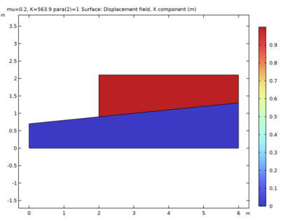
Figure 3 below shows the result for the case μ = 0.2, K = 563.9 N/m, and Figure 4 shows the contact pressure and friction forces for the same case. Both figures show the results obtained with the penalty method..
Figure 3: A surface plot of the x-displacement of the contactor wedge.
Figure 4: Contact pressure and friction forces acting on the contactor wedge.
Notes About the COMSOL Implementation
The initial unloaded state of the model is unstable and cause difficulties for the solver to find an initial solution. To avoid this issue, the first parameter step is set to 0.001. For this parameter value, a small amount of friction forces are present that stabilize the model.
The penalty method is not ideal for the type of large sliding problem with friction modeled in this example. While it in the limit will converge to the correct solution, the problem is stiff and ill-conditioned, meaning that small changes in the input can cause large changes to the results or even lead to no solution being found. In this example, the default solver suggestion does not give a stable solution, and the solver settings are modified to obtain a correct solution. Even with the modified settings, a warning from the linear solver gives an indication that the problem is ill-conditioned.
Reference
1. Feng Q., NAFEMS Benchmark Tests for Finite Element Modelling of Contact, Gapping and Sliding. NAFEMS Ref. R0081, UK, 2001.
Application Library path: Structural_Mechanics_Module/Verification_Examples/sliding_wedge
Modeling Instructions
From the File menu, choose New.
New
In the New window, click  Model Wizard.
Model Wizard
1
In the Model Wizard window, click  2D.
2
In the Select Physics tree, select Structural Mechanics>Solid Mechanics (solid).
3
Click Add.
4
Click  Study.
5
In the Select Study tree, select General Studies>Stationary.
6
Global Definitions
Parameters 1
1
In the Model Builder window, under Global Definitions click Parameters 1.
2
In the Settings window for Parameters, locate the Parameters section.
3
Geometry 1
Polygon 1 (pol1)
1
In the Geometry toolbar, click  Polygon.
2
In the Settings window for Polygon, locate the Coordinates section.
3
4
Click  Build All Objects.
Rectangle 1 (r1)
1
In the Geometry toolbar, click  Rectangle.
2
In the Settings window for Rectangle, locate the Size and Shape section.
3
In the Width text field, type 4.
4
In the Height text field, type 1.2.
5
Locate the Position section. In the x text field, type 1.
6
In the y text field, type 0.8.
Copy 1 (copy1)
1
In the Geometry toolbar, click  Transforms and choose Copy.
2
3
In the Settings window for Copy, click  Build Selected.
Difference 1 (dif1)
1
In the Geometry toolbar, click  Booleans and Partitions and choose Difference.
2
3
In the Settings window for Difference, locate the Difference section.
4
Find the Objects to subtract subsection. Click to select the  Activate Selection toggle button.
5
6
Click  Build Selected.
Form Union (fin)
1
In the Model Builder window, under Component 1 (comp1)>Geometry 1 click Form Union (fin).
2
In the Settings window for Form Union/Assembly, locate the Form Union/Assembly section.
3
From the Action list, choose Form an assembly.
4
From the Pair type list, choose Contact pair.
5
Click  Build Selected.
6
Click the  Zoom Extents button in the Graphics toolbar.
Materials
Material 1 (mat1)
1
In the Model Builder window, under Component 1 (comp1) right-click Materials and choose Blank Material.
2
In the Settings window for Material, locate the Material Contents section.
3
Solid Mechanics (solid)
Contact 1
In the Model Builder window, under Component 1 (comp1)>Solid Mechanics (solid) click Contact 1.
Friction 1
1
In the Physics toolbar, click  Attributes and choose Friction.
2
In the Settings window for Friction, locate the Friction Parameters section.
3
In the μ text field, type mu.
4
Locate the Initial Value section. From the Previous contact state list, choose In contact.
Body Load 1
1
In the Physics toolbar, click  Domains and choose Body Load.
2
3
In the Settings window for Body Load, locate the Force section.
4
From the Load type list, choose Total force.
5
Specify the Ftot vector as
Spring Foundation 1
1
In the Physics toolbar, click  Boundaries and choose Spring Foundation.
2
3
In the Settings window for Spring Foundation, locate the Spring section.
4
From the Spring type list, choose Total spring constant.
5
6
In the ktot table, enter the following settings:
Boundary Load 1
1
In the Physics toolbar, click  Boundaries and choose Boundary Load.
2
3
In the Settings window for Boundary Load, locate the Force section.
4
From the Load type list, choose Total force.
5
Specify the Ftot vector as
Fixed Constraint 1
1
In the Physics toolbar, click  Boundaries and choose Fixed Constraint.
2
Mesh 1
Mapped 1
In the Mesh toolbar, click  Mapped.
Distribution 1
1
Right-click Mapped 1 and choose Distribution.
2
3
In the Settings window for Distribution, locate the Distribution section.
4
In the Number of elements text field, type 10.
Distribution 2
1
In the Model Builder window, right-click Mapped 1 and choose Distribution.
2
3
In the Settings window for Distribution, locate the Distribution section.
4
In the Number of elements text field, type 60.
Distribution 3
1
Right-click Mapped 1 and choose Distribution.
2
3
In the Settings window for Distribution, locate the Distribution section.
4
In the Number of elements text field, type 40.
5
Click  Build All.
Study 1
Parametric Sweep
1
In the Study toolbar, click  Parametric Sweep.
2
In the Settings window for Parametric Sweep, locate the Study Settings section.
3
4
5
6
Step 1: Stationary
Set up an auxiliary continuation sweep for the para parameter.
1
In the Model Builder window, click Step 1: Stationary.
2
In the Settings window for Stationary, click to expand the Study Extensions section.
3
Select the Auxiliary sweep check box.
4
5
Set a stricter tolerance and tune the parameter stepping of the auxiliary sweep to improve the convergence of the model. The convergence is also improved by changing the nonlinear solver to Constant Newton.
Solution 1 (sol1)
1
In the Study toolbar, click  Show Default Solver.
2
In the Model Builder window, expand the Solution 1 (sol1) node, then click Stationary Solver 1.
3
In the Settings window for Stationary Solver, locate the General section.
4
In the Relative tolerance text field, type 1e-6.
5
In the Model Builder window, expand the Study 1>Solver Configurations>Solution 1 (sol1)>Stationary Solver 1 node, then click Parametric 1.
6
In the Settings window for Parametric, click to expand the Continuation section.
7
Select the Tuning of step size check box.
8
In the Initial step size text field, type 1e-2.
9
In the Minimum step size text field, type 1e-6.
10
From the Predictor list, choose Linear.
11
In the Model Builder window, under Study 1>Solver Configurations>Solution 1 (sol1)>Stationary Solver 1 click Fully Coupled 1.
12
In the Settings window for Fully Coupled, click to expand the Method and Termination section.
13
From the Nonlinear method list, choose Constant (Newton).
14
In the Model Builder window, click Study 1.
15
In the Settings window for Study, type Study 1: Penalty in the Label text field.
16
In the Study toolbar, click  Compute.
Results
Displacement: Penalty
In the Settings window for 2D Plot Group, type Displacement: Penalty in the Label text field.
Surface 1
1
In the Model Builder window, expand the Displacement: Penalty node, then click Surface 1.
2
In the Settings window for Surface, click Replace Expression in the upper-right corner of the Expression section. From the menu, choose Component 1 (comp1)>Solid Mechanics>Displacement>Displacement field - m>u - Displacement field, X component.
3
Locate the Coloring and Style section. From the Color table list, choose RainbowLight.
4
In the Displacement: Penalty toolbar, click  Plot.
5
Click the  Zoom Extents button in the Graphics toolbar.
Applied Loads: Penalty
1
In the Model Builder window, under Results click Applied Loads (solid).
2
In the Settings window for Group, type Applied Loads: Penalty in the Label text field.
Contact: Penalty
1
In the Model Builder window, under Results click Contact Forces (solid).
2
In the Settings window for 2D Plot Group, type Contact: Penalty in the Label text field.
Gray Surfaces
1
In the Model Builder window, expand the Contact: Penalty node, then click Gray Surfaces.
2
In the Contact: Penalty toolbar, click  Plot.
3
Click the  Zoom Extents button in the Graphics toolbar.
Follow the instructions below to evaluate the horizontal displacement for all three friction cases.
Point Evaluation: Penalty
1
In the Results toolbar, click  Point Evaluation.
2
In the Settings window for Point Evaluation, type Point Evaluation: Penalty in the Label text field.
3
Locate the Data section. From the Dataset list, choose Study 1: Penalty/Parametric Solutions 1 (sol2).
4
From the Parameter selection (para) list, choose Last.
5
From the Table columns list, choose mu, K.
6
7
Click Replace Expression in the upper-right corner of the Expressions section. From the menu, choose Component 1 (comp1)>Solid Mechanics>Displacement>Displacement field - m>u - Displacement field, X component.
8
Click  Evaluate.
Now, solve the model using the augmented Lagrangian formulation. Explore both a segregated and a coupled solution method.
Solid Mechanics (solid)
Contact 2
1
In the Model Builder window, under Component 1 (comp1)>Solid Mechanics (solid) right-click Contact 1 and choose Duplicate.
2
In the Settings window for Contact, locate the Pair Selection section.
3
Under Pairs, click  Add.
4
In the Add dialog box, select Contact Pair 1 (ap1) in the Pairs list.
5
6
In the Settings window for Contact, locate the Contact Method section.
7
From the Formulation list, choose Augmented Lagrangian.
Contact 3
1
Right-click Contact 2 and choose Duplicate.
2
In the Settings window for Contact, locate the Contact Method section.
3
From the Solution method list, choose Fully coupled.
Add Study
1
In the Home toolbar, click  Add Study to open the Add Study window.
2
Go to the Add Study window.
3
Find the Studies subsection. In the Select Study tree, select General Studies>Stationary.
4
5
In the Home toolbar, click  Add Study to close the Add Study window.
Study 2
Parametric Sweep
1
In the Study toolbar, click  Parametric Sweep.
2
In the Settings window for Parametric Sweep, locate the Study Settings section.
3
4
5
6
Step 1: Stationary
1
In the Model Builder window, click Step 1: Stationary.
2
In the Settings window for Stationary, locate the Physics and Variables Selection section.
3
Select the Modify model configuration for study step check box.
4
In the tree, select Component 1 (Comp1)>Solid Mechanics (Solid)>Contact 3.
5
6
Locate the Study Extensions section. Select the Auxiliary sweep check box.
7
8
9
In the Model Builder window, click Study 2.
10
In the Settings window for Study, type Study 2: Augmented Lagrangian, Segregated in the Label text field.
In this example the contact forces are very small, so it is necessary so set proper scales for these variables.
Solution 6 (sol6)
1
In the Study toolbar, click  Show Default Solver.
2
In the Model Builder window, expand the Solution 6 (sol6) node.
3
In the Model Builder window, expand the Study 2: Augmented Lagrangian, Segregated>Solver Configurations>Solution 6 (sol6)>Dependent Variables 1 node, then click Friction force (spatial frame) (comp1.solid.Tt_ap1).
4
In the Settings window for Field, locate the Scaling section.
5
In the Scale text field, type 100.
6
In the Model Builder window, under Study 2: Augmented Lagrangian, Segregated>Solver Configurations>Solution 6 (sol6)>Dependent Variables 1 click Contact pressure (comp1.solid.Tn_ap1).
7
In the Settings window for Field, locate the Scaling section.
8
In the Scale text field, type 1000.
9
In the Model Builder window, expand the Study 2: Augmented Lagrangian, Segregated>Solver Configurations>Solution 6 (sol6)>Stationary Solver 1 node, then click Parametric 1.
10
In the Settings window for Parametric, locate the Continuation section.
11
Select the Tuning of step size check box.
12
In the Initial step size text field, type 0.1.
13
In the Maximum step size text field, type 1.
14
In the Study toolbar, click  Compute.
Similarly, add a third study for the augmented Lagrangian formulation with a coupled solution method and compute the solution. Disable Contact 1 and Contact 2, and use a Constant (Newton) solver.
Results
Displacement: Augmented Lagrangian, Segregated
In the Settings window for 2D Plot Group, type Displacement: Augmented Lagrangian, Segregated in the Label text field.
Surface 1
1
In the Model Builder window, expand the Displacement: Augmented Lagrangian, Segregated node, then click Surface 1.
2
In the Settings window for Surface, click Replace Expression in the upper-right corner of the Expression section. From the menu, choose Component 1 (comp1)>Solid Mechanics>Displacement>Displacement field - m>u - Displacement field, X component.
3
Locate the Coloring and Style section. From the Color table list, choose RainbowLight.
4
In the Displacement: Augmented Lagrangian, Segregated toolbar, click  Plot.
5
Click the  Zoom Extents button in the Graphics toolbar.
Applied Loads: Augmented Lagrangian, Segregated
1
In the Model Builder window, under Results click Applied Loads (solid).
2
In the Settings window for Group, type Applied Loads: Augmented Lagrangian, Segregated in the Label text field.
Contact: Augmented Lagrangian, Segregated
1
In the Model Builder window, under Results click Contact Forces (solid).
2
In the Settings window for 2D Plot Group, type Contact: Augmented Lagrangian, Segregated in the Label text field.
Gray Surfaces
1
In the Model Builder window, expand the Contact: Augmented Lagrangian, Segregated node, then click Gray Surfaces.
2
In the Contact: Augmented Lagrangian, Segregated toolbar, click  Plot.
3
Click the  Zoom Extents button in the Graphics toolbar.
Point Evaluation: Augmented Lagrangian, Segregated
1
In the Model Builder window, right-click Point Evaluation: Penalty and choose Duplicate.
2
In the Settings window for Point Evaluation, type Point Evaluation: Augmented Lagrangian, Segregated in the Label text field.
3
Locate the Data section. From the Dataset list, choose Study 2: Augmented Lagrangian, Segregated/Parametric Solutions 2 (sol7).
4
Clicknext to  Evaluate, then choose New Table.
Repeat the same steps for the datasets and plots generated by Study 3: Augmented Lagrangian, Coupled.
Prepare the model for later use by disabling the second and third contact nodes in Study 1: Penalty.
Study 1: Penalty
Step 1: Stationary
1
In the Model Builder window, under Study 1: Penalty click Step 1: Stationary.
2
In the Settings window for Stationary, locate the Physics and Variables Selection section.
3
Select the Modify model configuration for study step check box.
4
In the tree, select Component 1 (Comp1)>Solid Mechanics (Solid)>Contact 2.
5
6
In the tree, select Component 1 (Comp1)>Solid Mechanics (Solid)>Contact 3.
7