PDF

Micromechanical Model of a Composite
Introduction
The use of fiber reinforced composites is increasing in various industries like automotive, aerospace, infrastructure, and many more. The accuracy of structural or thermal analysis relies on an accurate estimation of mechanical and thermal properties of the composite material.
In this example, a simplified micromechanical model of a unit cell with periodic boundary conditions is analyzed. The unit cell is a representative volume element (RVE) which repeats itself to form the complete structure of the composite. In the current model, the unit cell is made of a single carbon fiber placed at center of an epoxy matrix. The fiber volume fraction is varied. The homogenized elastic and thermal properties of the composite material are computed based on the individual properties of fiber and matrix. A comparison is made against values obtained from the Rule of Mixture (ROM).
Model Definition
The composite is assumed to be made of carbon fibers unidirectionally embedded in epoxy resin. A representative unit cell having a cylindrical fiber located at the center of resin is shown in Figure 1. The fiber radius is computed based on a parameterized fiber volume fraction.
Figure 1: Geometry of the unit cell with a carbon fiber in an epoxy resin.
Fiber and Matrix Properties
The layers of the laminate are made of T300 carbon fiber and 914C epoxy. The carbon fiber is assumed to be transversely isotropic (modeled as orthotropic), and the epoxy resin is assumed to be isotropic. The material properties of fiber and resin are given in Table 1 and Table 2 respectively.
{E1f,E2f,E3f}
{G12f,G23f,G13f}
{15,7,15} (GPa)
{υ12f,υ23f,υ13f}
ρf
1800 (kg/m3)
Em
4 (GPa)
υm
ρm
1100 (kg/m3)
For computing homogeneous elastic properties, the Poisson’s ratios for the fiber and matrix materials are intentionally set to zero, in order to reduce the elements of elasticity matrix D11, D22, D33 to homogenized Young’s modulus E11, E22, E33 respectively. In this way, results can be easily compared to the homogenized Young’s moduli computed with the ROM.
The homogeneous thermal properties are computed with zero Poisson’s ratio as well as with the ratios given in Table 1 and Table 2.
Rule of Mixture (ROM)
Based on the material properties from Table 1 and Table 2, the homogenized Young’s moduli, the in-plane shear modulus, and the in-plane Poisson’s ratio are computed from the ROM as (Ref. 1):
(1)
(2)
(3)
(4)
Here, Vf and Vm are the fiber and matrix volume fractions, respectively. The coefficients of thermal expansion for a composite in the fiber and transverse directions are calculated from the rule of mixture using:
(5)
(6)
The above formulas are used to compute analytical values of the homogenized elastic and thermal properties for comparison with the RVE model.
Results and Discussion
Figure 2 and Figure 3 show the comparison between the longitudinal and transversal homogeneous Young’s moduli computed from the RVE and the ROM. The longitudinal Young’s modulus matches quite closely. The transverse Young’s modulus, however, differs more and more as fiber volume fraction increases. The same behavior is observed for the in-plane homogeneous shear modulus (Figure 4). This is not surprising, given that the transverse stresses are much more inhomogeneous than those along the fiber.
Figure 2: Longitudinal Young's modulus versus fiber volume fraction.
Figure 3: Transverse Young's modulus versus fiber volume fraction..
Figure 4: In-plane shear modulus versus fiber volume fraction.
The longitudinal and transverse homogeneous coefficients of thermal expansion computed using the RVE and the ROM are shown in the Figure 5 and Figure 6, respectively for zero Poisson’s ratio. As expected, the longitudinal coefficient of thermal expansion matches exactly, while the numerically computed transverse coefficient of thermal expansion differs from the prediction by the ROM.
For nonzero Poisson’s ratio, the homogeneous longitudinal and transverse coefficients of thermal expansion are shown in Figure 7 and Figure 8, respectively. Now, the numerically computed longitudinal coefficient of thermal expansion no longer matches the ROM values. The same behavior can also be expected for the longitudinal Young’s modulus.
All figures indicate that the macromechanically computed longitudinal elastic and thermal properties match exactly with the values computed from the ROM when the constituent materials have zero Poisson’s ratio. For nonzero Poisson’s ratio, even longitudinal properties computed numerically and from the ROM differ.
The transverse/shear elastic and thermal properties do not match well with the values computed from the ROM. The difference increases with increasing fiber volume fraction.
Figure 5: Longitudinal coefficient of thermal expansion versus fiber volume fraction.
Figure 6: Transverse coefficient of thermal expansion versus fiber volume fraction.
Figure 7: Longitudinal coefficient of thermal expansion versus fiber volume fraction with nonzero Poisson’s ratio.
Figure 8: Transverse coefficient of thermal expansion versus fiber volume fraction with nonzero Poisson’s ratio.
Notes About the COMSOL Implementation
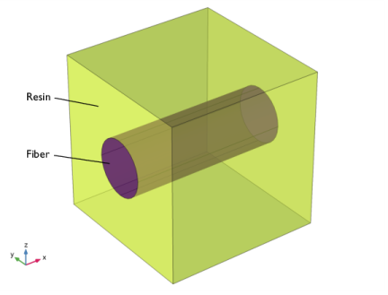
In order to perform a micromechanical analysis, the Cell Periodicity node in the Solid Mechanics interface is used. The Cell Periodicity node is used to apply periodic boundary conditions to the three pairs of faces of the unit cell.
In order to extract the homogenized elasticity matrix for a composite, the Average strain periodicity type needs to be chosen. The unit cell needs to be analyzed for six different load cases. This is automatically done through the Cell Periodicity node by clicking the Create button. This operation adds the required number of load cases, populates the average strain matrix with boolean variables, creates a global material, and creates a stationary study with preselected load groups. The created global material contains an elasticity matrix corresponding to that of the homogenized material. This material can be used to define the properties of individual layers in a composite laminate. If, by mistake, one of the automatically generated nodes is edited or deleted, you can click the Create button again to regenerate those nodes.
The default computed homogenized elasticity matrix D is tied to the tag of the solution node of an automatically generated study. In this example, D is computed in a parametric sweep. The elements of elasticity matrix must then be accessed using customized expressions as the tag of the parametric solution node is different.
In order to extract the homogenized coefficient of thermal expansions, the Free Expansion option with Coefficient of thermal expansion is used.
Reference
1. N. Srisuk, A Micromechanics Model of Thermal Expansion Coefficient in Fiber Reinforced Composites, Master Thesis-The University of Texas st Arlington, 2010.
Application Library path: Structural_Mechanics_Module/Material_Models/micromechanical_model_of_a_composite
Modeling Instructions
From the File menu, choose New.
New
In the New window, click  Model Wizard.
Model Wizard
1
In the Model Wizard window, click  3D.
2
In the Select Physics tree, select Structural Mechanics>Solid Mechanics (solid).
3
Click Add.
4
Global Definitions
Parameters 1
1
In the Model Builder window, under Global Definitions click Parameters 1.
2
In the Settings window for Parameters, locate the Parameters section.
3
Click  Load from File.
4
Geometry 1
Block: Resin
1
In the Geometry toolbar, click  Block.
2
In the Settings window for Block, type Block: Resin in the Label text field.
3
Locate the Size and Shape section. In the Width text field, type l.
4
In the Depth text field, type l.
5
In the Height text field, type l.
6
Locate the Selections of Resulting Entities section. Select the Resulting objects selection check box.
7
From the Color list, choose Color 4.
On Windows, click the 4th color in the first row of the palette.
Cylinder: Fiber
1
In the Geometry toolbar, click  Cylinder.
2
In the Settings window for Cylinder, type Cylinder: Fiber in the Label text field.
3
Locate the Size and Shape section. In the Radius text field, type r_f.
4
In the Height text field, type l.
5
Locate the Position section. In the y text field, type l/2.
6
In the z text field, type l/2.
7
Locate the Axis section. From the Axis type list, choose x-axis.
8
Locate the Selections of Resulting Entities section. Select the Resulting objects selection check box.
9
From the Color list, choose Color 1.
On Windows, click the 1st color in the first row of the palette.
10
In the Geometry toolbar, click  Build All.
Solid Mechanics (solid)
Linear Elastic Material 1
In the Model Builder window, under Component 1 (comp1)>Solid Mechanics (solid) click Linear Elastic Material 1.
Thermal Expansion 1
1
In the Physics toolbar, click  Attributes and choose Thermal Expansion.
2
In the Settings window for Thermal Expansion, locate the Model Input section.
3
From the T list, choose User defined. In the associated text field, type 21[degC].
Linear Elastic Material 2
1
In the Physics toolbar, click  Domains and choose Linear Elastic Material.
2
3
In the Settings window for Linear Elastic Material, locate the Linear Elastic Material section.
4
From the Solid model list, choose Orthotropic.
Thermal Expansion 1
1
In the Physics toolbar, click  Attributes and choose Thermal Expansion.
2
In the Settings window for Thermal Expansion, locate the Model Input section.
3
From the T list, choose User defined. In the associated text field, type 21[degC].
Cell Periodicity for Elastic Properties
1
In the Physics toolbar, click  Domains and choose Cell Periodicity.
2
In the Settings window for Cell Periodicity, type Cell Periodicity for Elastic Properties in the Label text field.
3
Locate the Domain Selection section. From the Selection list, choose All domains.
4
Locate the Periodicity Type section. From the list, choose Average strain.
5
From the Calculate average properties list, choose Elasticity matrix, Standard (XX, YY, ZZ, XY, YZ, XZ).
Boundary Pair 1
1
In the Physics toolbar, click  Attributes and choose Boundary Pair.
2
In the Settings window for Boundary Pair, locate the Boundary Selection section.
3
Click  Clear Selection.
4
Boundary Pair 2
1
Right-click Boundary Pair 1 and choose Duplicate.
2
In the Settings window for Boundary Pair, locate the Boundary Selection section.
3
Click  Clear Selection.
4
Boundary Pair 3
1
Right-click Boundary Pair 2 and choose Duplicate.
2
In the Settings window for Boundary Pair, locate the Boundary Selection section.
3
Click  Clear Selection.
4
With the Average strain option in the Cell Periodicity feature, appropriate load groups, a study and a material with computed elastic properties can be generated automatically. To create load groups and a study node, click the Create Load Groups and Study button in the section toolbar.
Cell Periodicity for Elastic Properties
1
In the Model Builder window, click Cell Periodicity for Elastic Properties.
2
In the Settings window for Cell Periodicity, locate the Periodicity Type section.
3
Click Create Load Groups and Study in the upper-right corner of the section.
Cell Periodicity for Thermal Properties
1
Right-click Cell Periodicity for Elastic Properties and choose Duplicate.
2
In the Settings window for Cell Periodicity, type Cell Periodicity for Thermal Properties in the Label text field.
3
Locate the Periodicity Type section. From the list, choose Free expansion.
4
From the Calculate average properties list, choose Coefficient of thermal expansion.
Materials
Material 1: Epoxy Resin
1
In the Model Builder window, under Component 1 (comp1) right-click Materials and choose Blank Material.
2
In the Settings window for Material, type Material 1: Epoxy Resin in the Label text field.
3
4
Locate the Material Contents section. In the table, enter the following settings:
Material 2: Carbon Fiber
1
Right-click Materials and choose Blank Material.
2
In the Settings window for Material, type Material 2: Carbon Fiber in the Label text field.
3
Locate the Geometric Entity Selection section. Click  Paste Selection.
4
In the Paste Selection dialog box, type 2 in the Selection text field.
5
6
In the Settings window for Material, locate the Material Contents section.
7
Mesh 1
Free Triangular 1
1
In the Mesh toolbar, click  Boundary and choose Free Triangular.
2
3
In the Settings window for Free Triangular, click  Build Selected.
Swept 1
1
In the Mesh toolbar, click  Swept.
2
In the Settings window for Swept, click  Build Selected.
For this study, disable the thermal expansion nodes and the cell periodicity feature for thermal expansion.
Cell Periodicity Study for Elastic Properties
1
In the Model Builder window, click Cell Periodicity Study.
2
In the Settings window for Study, type Cell Periodicity Study for Elastic Properties in the Label text field.
Parametric Sweep
1
In the Study toolbar, click  Parametric Sweep.
2
In the Settings window for Parametric Sweep, locate the Study Settings section.
3
4
Step 1: Stationary
1
In the Model Builder window, click Step 1: Stationary.
2
In the Settings window for Stationary, locate the Physics and Variables Selection section.
3
Select the Modify model configuration for study step check box.
4
In the tree, select Component 1 (Comp1)>Solid Mechanics (Solid)>Linear Elastic Material 1>Thermal Expansion 1.
5
6
In the tree, select Component 1 (Comp1)>Solid Mechanics (Solid)>Linear Elastic Material 2>Thermal Expansion 1.
7
8
In the tree, select Component 1 (Comp1)>Solid Mechanics (Solid)>Cell Periodicity for Thermal Properties.
9
The default computed homogenized elasticity matrix D is tied to the tag of the solution node of the automatically generated study. Hence, if one needs to compute D matrix with a parametric sweep, the elements of the elasticity matrix need to be computed using customized expressions, as the tag of the parametric solution node is different.
Create a Variable node and enter the following customized expressions to compute the elements of the D matrix for postprocessing purpose.
Definitions
Variables 1
1
In the Model Builder window, under Component 1 (comp1) right-click Definitions and choose Variables.
2
In the Settings window for Variables, locate the Variables section.
3
Cell Periodicity Study for Elastic Properties
In the Study toolbar, click  Compute.
Add a separate study to compute the homogeneous thermal properties. For this study, disable the cell periodicity feature for elastic properties.
Add Study
1
In the Study toolbar, click  Add Study to open the Add Study window.
2
Go to the Add Study window.
3
Find the Studies subsection. In the Select Study tree, select General Studies>Stationary.
4
5
In the Study toolbar, click  Add Study to close the Add Study window.
Cell Periodicity Study for Thermal Properties
In the Settings window for Study, type Cell Periodicity Study for Thermal Properties in the Label text field.
Parametric Sweep
1
In the Study toolbar, click  Parametric Sweep.
This study computes the homogenized thermal properties with zero and nonzero Poisson’s ratios. Therefore, use a parametric sweep for the parameter para along with v_f.
2
In the Settings window for Parametric Sweep, locate the Study Settings section.
3
From the Sweep type list, choose All combinations.
4
5
6
7
Step 1: Stationary
1
In the Model Builder window, click Step 1: Stationary.
2
In the Settings window for Stationary, locate the Physics and Variables Selection section.
3
Select the Modify model configuration for study step check box.
4
In the tree, select Component 1 (Comp1)>Solid Mechanics (Solid)>Cell Periodicity for Elastic Properties.
5
6
In the Study toolbar, click  Compute.
When plotting the computed elasticity matrix elements in 1D plot groups, the load case in the parameter selection is irrelevant.
Results
Longitudinal Young’s Modulus vs. Fiber Volume Fraction
1
In the Home toolbar, click  Add Plot Group and choose 1D Plot Group.
2
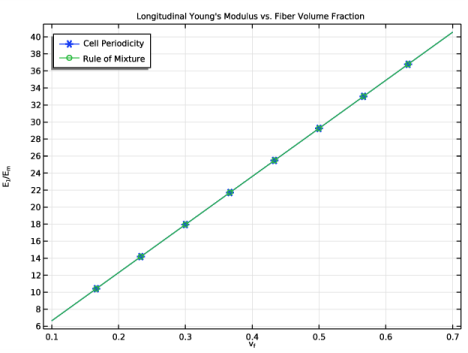
In the Settings window for 1D Plot Group, type Longitudinal Young's Modulus vs. Fiber Volume Fraction in the Label text field.
3
Locate the Data section. From the Dataset list, choose Cell Periodicity Study for Elastic Properties/Parametric Solutions 1 (sol1).
4
From the Parameter selection (Load case) list, choose First.
5
Click to expand the Title section. From the Title type list, choose Manual.
6
In the Title text area, type Longitudinal Young's Modulus vs. Fiber Volume Fraction.
7
Locate the Plot Settings section. Select the x-axis label check box.
8
9
Select the y-axis label check box.
10
In the associated text field, type E<sub>1</sub>/E<sub>m</sub>.
11
Locate the Legend section. From the Position list, choose Upper left.
Global 1
1
Right-click Longitudinal Young’s Modulus vs. Fiber Volume Fraction and choose Global.
2
In the Settings window for Global, locate the y-Axis Data section.
3
4
Locate the x-Axis Data section. From the Axis source data list, choose v_f.
5
Click to expand the Coloring and Style section. Find the Line markers subsection. From the Marker list, choose Cycle.
6
Click to expand the Legends section. From the Legends list, choose Manual.
7
8
Longitudinal Coefficient of Thermal Expansion vs. Fiber Volume Fraction
1
In the Model Builder window, right-click Longitudinal Young’s Modulus vs. Fiber Volume Fraction and choose Duplicate.
2
In the Settings window for 1D Plot Group, locate the Data section.
3
From the Dataset list, choose Cell Periodicity Study for Thermal Properties/Parametric Solutions 2 (sol10).
4
From the Parameter selection (para) list, choose From list.
5
In the Parameter values (para) list, select 0.
6
From the Parameter selection (v_f) list, choose All.
7
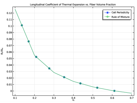
In the Label text field, type Longitudinal Coefficient of Thermal Expansion vs. Fiber Volume Fraction.
8
Locate the Title section. In the Title text area, type Longitudinal Coefficient of Thermal Expansion vs. Fiber Volume Fraction.
9
Locate the Plot Settings section. In the y-axis label text field, type \alpha<sub>1</sub>/\alpha<sub>m</sub>.
10
Locate the Legend section. From the Position list, choose Upper right.
Global 1
1
In the Model Builder window, expand the Longitudinal Coefficient of Thermal Expansion vs. Fiber Volume Fraction node, then click Global 1.
2
In the Settings window for Global, click Replace Expression in the upper-right corner of the y-Axis Data section. From the menu, choose Component 1 (comp1)>Solid Mechanics>Cell periodicity>Coefficient of thermal expansion (material and geometry frames) - 1/K>solid.cp2.alphaXX - Coefficient of thermal expansion, XX component.
3
Locate the y-Axis Data section. In the table, enter the following settings:
4
Locate the x-Axis Data section. From the Axis source data list, choose v_f.
5
In the Longitudinal Coefficient of Thermal Expansion vs. Fiber Volume Fraction toolbar, click  Plot.
6
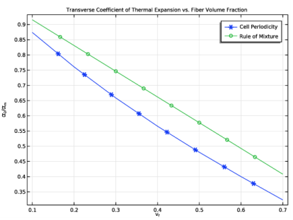
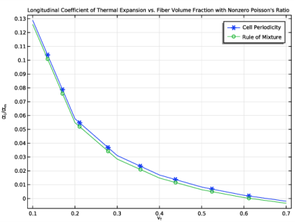
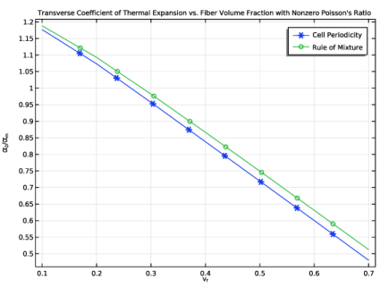
Duplicate or add this plot group three times in order to plot the remaining thermal properties. The labels, titles, parameter values, and expressions to be defined in the Global 1 node are shown in the table below. The parameter value of para needs to be changed in the Data section of the corresponding 1D plot group.
You can finally group the plots for better readability.
In-plane Shear Modulus vs. Fiber Volume Fraction, Longitudinal Young’s Modulus vs. Fiber Volume Fraction, Transverse Young’s Modulus vs. Fiber Volume Fraction
1
In the Model Builder window, under Results, Ctrl-click to select Longitudinal Young’s Modulus vs. Fiber Volume Fraction, Transverse Young’s Modulus vs. Fiber Volume Fraction, and In-plane Shear Modulus vs. Fiber Volume Fraction.
2
Elastic Properties
In the Settings window for Group, type Elastic Properties in the Label text field.
Longitudinal Coefficient of Thermal Expansion vs. Fiber Volume Fraction, Transverse Coefficient of Thermal Expansion vs. Fiber Volume Fraction
1
In the Model Builder window, under Results, Ctrl-click to select Longitudinal Coefficient of Thermal Expansion vs. Fiber Volume Fraction and Transverse Coefficient of Thermal Expansion vs. Fiber Volume Fraction.
2
Thermal Expansion Properties, Zero Poisson’s Ratio
In the Settings window for Group, type Thermal Expansion Properties, Zero Poisson's Ratio in the Label text field.
Longitudinal Coefficient of Thermal Expansion vs. Fiber Volume Fraction with Nonzero Poisson’s Ratio, Transverse Coefficient of Thermal Expansion vs. Fiber Volume Fraction with Nonzero Poisson’s Ratio
1
In the Model Builder window, under Results, Ctrl-click to select Longitudinal Coefficient of Thermal Expansion vs. Fiber Volume Fraction with Nonzero Poisson’s Ratio and Transverse Coefficient of Thermal Expansion vs. Fiber Volume Fraction with Nonzero Poisson’s Ratio.
2
Thermal Expansion Properties, Nonzero Poisson’s Ratio
In the Settings window for Group, type Thermal Expansion Properties, Nonzero Poisson's Ratio in the Label text field.