|
|
|

|
•
|
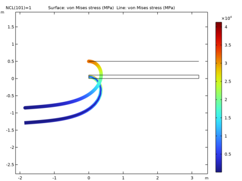
The length of the beam is 3.2 m.
|
|
•
|

|
1
|
|
2
|
|
3
|
Click Add.
|
|
4
|
|
5
|
Click Add.
|
|
6
|
Click
|
|
7
|
|
8
|
Click
|
|
1
|
|
2
|
|
3
|
|
4
|
Browse to the model’s Application Libraries folder and double-click the file large_deformation_beam_parameters.txt.
|
|
1
|
|
2
|
|
3
|
|
4
|
|
1
|
|
2
|
|
4
|
|
1
|
|
2
|
|
1
|
In the Model Builder window, under Global Definitions right-click Materials and choose Blank Material.
|
|
2
|
|
3
|
|
4
|
|
5
|
|
6
|
|
7
|
|
8
|
|
9
|
|
1
|
|
2
|
|
3
|
|
1
|
|
2
|
|
3
|
|
4
|
|
1
|
|
1
|
|
3
|
|
4
|
|
5
|
|
1
|
|
2
|
|
3
|
|
1
|
|
2
|
|
3
|
|
4
|
|
5
|
|
1
|
|
1
|
|
2
|
|
3
|
|
1
|
|
2
|
|
3
|
|
1
|
|
1
|
|
2
|
|
3
|
|
5
|
|
1
|
|
2
|
|
3
|
|
5
|
|
1
|
|
2
|
|
1
|
|
2
|
|
3
|
|
4
|
Locate the Physics and Variables Selection section. Select the Modify model configuration for study step check box.
|
|
5
|
|
6
|
Click
|
|
7
|
|
8
|
Click
|
|
10
|
|
1
|
In the Model Builder window, expand the Study 1>Solver Configurations>Solution 1 (sol1) node, then click Stationary Solver 1.
|
|
2
|
|
3
|
|
4
|
In the Model Builder window, expand the Study 1>Solver Configurations>Solution 1 (sol1)>Stationary Solver 1 node.
|
|
5
|
|
6
|
|
7
|
|
8
|
In the Model Builder window, expand the Study 1>Solver Configurations>Solution 1 (sol1)>Stationary Solver 1>Segregated 1 node, then click Segregated Step.
|
|
9
|
|
10
|
|
11
|
|
12
|
|
13
|
Click to expand the Method and Termination section. From the Termination technique list, choose Tolerance.
|
|
14
|
|
15
|
|
16
|
|
17
|
In the Add dialog box, in the Variables list, choose Rotation field (material and geometry frames) (comp1.beam.thLin) and Displacement field (material and geometry frames) (comp1.beam.uLin).
|
|
18
|
Click OK.
|
|
19
|
|
20
|
|
21
|
|
22
|
|
1
|
|
2
|
|
3
|
Select the Plot check box.
|
|
4
|
|
5
|
|
1
|
|
2
|
|
3
|
|
4
|
|
1
|
|
2
|
|
3
|
|
1
|
|
2
|
|
3
|
|
4
|
|
1
|
|
2
|
|
3
|
|
4
|
|
5
|
|
1
|
|
2
|
|
3
|
|
4
|
|
5
|
Click
|
|
6
|
|
1
|
|
2
|
|
3
|
|
1
|
|
2
|
In the Settings window for Point Graph, click Replace Expression in the upper-right corner of the y-Axis Data section. From the menu, choose Component 1 (comp1)>Solid Mechanics>Displacement>Displacement field - m>u - Displacement field, X component.
|
|
3
|
|
4
|
|
5
|
|
1
|
|
2
|
In the Settings window for Point Graph, click Replace Expression in the upper-right corner of the y-Axis Data section. From the menu, choose Component 1 (comp1)>Solid Mechanics>Displacement>Displacement field - m>v - Displacement field, Y component.
|
|
3
|
Locate the Coloring and Style section. Find the Line style subsection. From the Line list, choose Dashed.
|
|
4
|
|
5
|
|
6
|
|
1
|
|
2
|
|
3
|
|
4
|
|
6
|
Click Replace Expression in the upper-right corner of the y-Axis Data section. From the menu, choose Component 1 (comp1)>Beam>Displacement>Displacement field - m>u2 - Displacement field, X component.
|
|
7
|
Locate the Coloring and Style section. Find the Line style subsection. From the Line list, choose Dotted.
|
|
8
|
|
9
|
|
10
|
|
11
|
|
1
|
|
2
|
In the Settings window for Point Graph, click Replace Expression in the upper-right corner of the y-Axis Data section. From the menu, choose Component 1 (comp1)>Beam>Displacement>Displacement field - m>v2 - Displacement field, Y component.
|
|
3
|
Locate the Coloring and Style section. Find the Line markers subsection. From the Marker list, choose Circle.
|
|
4
|
Locate the Legends section. In the table, enter the following settings:
|
|
5
|
|
1
|
|
2
|
|
3
|
|
4
|
|
5
|
|
6
|
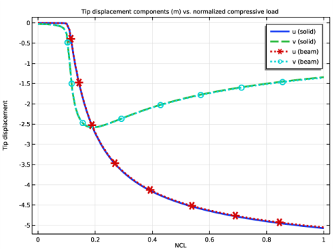
In the associated text field, type Tip displacement.
|
|
7
|
|
8
|
|
1
|
|
2
|
|
3
|
|
4
|
|
5
|
Click Replace Expression in the upper-right corner of the Expressions section. From the menu, choose Component 1 (comp1)>Solid Mechanics>Displacement>Displacement field - m>u - Displacement field, X component.
|
|
6
|
Locate the Expressions section. In the table, enter the following settings:
|
|
7
|
Click
|
|
1
|
|
2
|
|
3
|
|
4
|
|
6
|
Locate the Expressions section. In the table, enter the following settings:
|
|
7
|
|
1
|
In the Model Builder window, under Results>Derived Values right-click Point Evaluation 1 and choose Duplicate.
|
|
2
|
|
4
|
|
1
|
In the Model Builder window, under Results>Derived Values right-click Point Evaluation 2 and choose Duplicate.
|
|
2
|
|
4
|
|
1
|
In the Model Builder window, under Results>Derived Values right-click Point Evaluation 3 and choose Duplicate.
|
|
2
|
|
3
|
|
4
|
Locate the Expressions section. In the table, enter the following settings:
|
|
5
|
|
6
|
|
1
|
In the Model Builder window, under Results>Derived Values right-click Point Evaluation 4 and choose Duplicate.
|
|
2
|
|
3
|
|
4
|
Locate the Expressions section. In the table, enter the following settings:
|
|
5
|
|
6
|
|
1
|
|
2
|
|
3
|
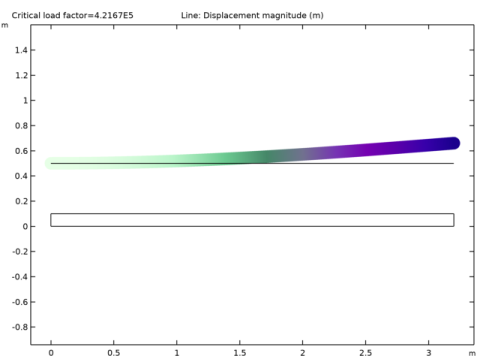
Find the Studies subsection. In the Select Study tree, select Preset Studies for Selected Physics Interfaces>Linear Buckling.
|
|
4
|
|
5
|
|
1
|
|
2
|
|
3
|
|
4
|
|
5
|
|
6
|
Click
|
|
1
|
|
2
|
|
3
|
|
4
|
|
5
|
|
6
|
|
7
|
Click
|
|
8
|
|
1
|
|
2
|
|
3
|
|
5
|
Locate the Expressions section. In the table, enter the following settings:
|
|
6
|
Click
|