PDF

In-Plane and Space Truss
Introduction
In the following example you first build and solve a simple 2D truss model using the 2D Truss interface. Later on, you analyze a 3D variant of the same problem using the 3D Truss interface. This model calculates the deformation and forces of a simple geometry. The example is based on problem 11.1 in Aircraft Structures for Engineering Students by T.H.G Megson (Ref. 1). The results are compared with the analytical results given in Ref. 1.
Model Definition
The 2D geometry consists of a square symmetrical truss built up by five members. All members have the same cross-sectional area A. The side length is L, and the Young’s modulus is E.
Figure 1: The truss geometry.
In the 3D case, another copy of the diagonal bars are rotated 90° around the vertical axis so that a cube with one space diagonal is generated. The figure above is thus applicable to a view in the zy-plane as well as in the xy-plane. The central bar is then given twice the area of the other members. In this way, a space truss with exactly the same type of symmetry, but twice the vertical stiffness is generated.
GEOMETRY
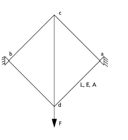
The truss members have a circular cross section with a radius of 0.05 m. In the 3D case, the area of the central bar is doubled.
Material
Aluminum: Young’s modulus, E = 70 GPa, Poisson’s ration ν = 0.3.
Constraints
In the 2D case, displacements in both directions are constrained at vertices a and b. In the 3D case, the two new points are constrained in the same way.
Load
In the 2D case, a vertical force F of 50 kN is applied at the bottom corner. In the 3D case, the value 100 kN is used instead in order to get the same displacements.
Results and Discussion
The following table shows a comparison between the results calculated with the Structural Mechanics Module and the analytical results from Ref. 1.
The results are in nearly perfect agreement.
Figure 2 and Figure 3 show plots visualizing the deformed geometry together with the axial forces in the truss members.
Figure 2: Deformed geometry and axial forces for the 2D case.
Figure 3: Deformed geometry and axial forces for the 3D case.
Notes About the COMSOL Implementation
In this example you build the 2D and the 3D truss as two different components within the same MPH file. This is not essential, you could equally well choose to create the components in separate MPH files.
Reference
1. T.H.G. Megson, Aircraft Structures for Engineering Students, Edward Arnold, p. 404, 1985
Application Library path: Structural_Mechanics_Module/Verification_Examples/inplane_and_space_truss
Modeling Instructions
From the File menu, choose New.
New
In the New window, click  Model Wizard.
Model Wizard
1
In the Model Wizard window, click  2D.
2
In the Select Physics tree, select Structural Mechanics>Truss (truss).
3
Click Add.
4
Click  Study.
5
In the Select Study tree, select General Studies>Stationary.
6
Geometry 1
Square 1 (sq1)
1
In the Geometry toolbar, click  Square.
2
In the Settings window for Square, locate the Size section.
3
In the Side length text field, type 2.
4
Locate the Rotation Angle section. In the Rotation text field, type 45.
5
Locate the Object Type section. From the Type list, choose Curve.
6
Click  Build All Objects.
7
Click the  Zoom Extents button in the Graphics toolbar.
Line Segment 1 (ls1)
1
In the Geometry toolbar, click  More Primitives and choose Line Segment.
2
In the Settings window for Line Segment, locate the Starting Point section.
3
From the Specify list, choose Coordinates.
4
Locate the Endpoint section. From the Specify list, choose Coordinates.
5
In the y text field, type sqrt(8).
6
Click  Build All Objects.
Truss (truss)
Cross-Section Data 1
1
In the Model Builder window, under Component 1 (comp1)>Truss (truss) click Cross-Section Data 1.
2
In the Settings window for Cross-Section Data, locate the Cross-Section Data section.
3
In the A text field, type pi/4*0.05^2.
Pinned 1
1
In the Physics toolbar, click  Points and choose Pinned.
2
Point Load 1
1
In the Physics toolbar, click  Points and choose Point Load.
2
3
In the Settings window for Point Load, locate the Force section.
4
Specify the FP vector as
Global Definitions
In this example, the same material data will be referenced from two different components, so it is convenient to define a global material.
Material 1 (mat1)
1
In the Model Builder window, under Global Definitions right-click Materials and choose Blank Material.
2
In the Settings window for Material, click to expand the Material Properties section.
3
In the Material properties tree, select Basic Properties>Density.
4
Click  Add to Material.
5
In the Material properties tree, select Solid Mechanics>Linear Elastic Material>Young’s Modulus and Poisson’s Ratio.
6
Click  Add to Material.
7
Locate the Material Contents section. In the table, enter the following settings:
Materials
Material Link 1 (matlnk1)
In the Model Builder window, under Component 1 (comp1) right-click Materials and choose More Materials>Material Link.
Study 1
In the Home toolbar, click  Compute.
Results
Force (truss)
1
In the Model Builder window, expand the Results>Force (truss) node, then click Force (truss).
2
In the Settings window for 2D Plot Group, locate the Color Legend section.
3
Select the Show maximum and minimum values check box.
4
Click the  Zoom Extents button in the Graphics toolbar.
Next, compute the displacements at d (Vertex 2) and c (Vertex 3).
Displacement of Vertices (2D)
1
In the Results toolbar, click  Evaluation Group.
2
In the Settings window for Evaluation Group, type Displacement of Vertices (2D) in the Label text field.
Point Evaluation 1
1
Right-click Displacement of Vertices (2D) and choose Point Evaluation.
2
3
In the Settings window for Point Evaluation, locate the Expressions section.
4
5
In the Displacement of Vertices (2D) toolbar, click  Evaluate.
Although you can read off the values of the local axial force in the members ac and ad from the max and min values for the color legend for the plot in the Graphics window, it is instructive to see how you can compute such values more generally.
Definitions
Add nonlocal average couplings for the members ac, ad, and cd. You will use these for defining variables that evaluate the axial forces in these members.
Average 1 (aveop1)
1
In the Definitions toolbar, click  Nonlocal Couplings and choose Average.
2
In the Settings window for Average, type aveop_ac in the Operator name text field.
3
Locate the Source Selection section. From the Geometric entity level list, choose Boundary.
4
Average 2 (aveop2)
1
In the Definitions toolbar, click  Nonlocal Couplings and choose Average.
2
In the Settings window for Average, type aveop_ad in the Operator name text field.
3
Locate the Source Selection section. From the Geometric entity level list, choose Boundary.
4
Average 3 (aveop3)
1
In the Definitions toolbar, click  Nonlocal Couplings and choose Average.
2
In the Settings window for Average, type aveop_cd in the Operator name text field.
3
Locate the Source Selection section. From the Geometric entity level list, choose Boundary.
4
Variables 1
1
In the Definitions toolbar, click  Local Variables.
2
In the Settings window for Variables, locate the Variables section.
3
Study 1
Update the solution to evaluate the variables you just defined.
Solution 1 (sol1)
1
In the Model Builder window, expand the Study 1>Solver Configurations node.
2
Right-click Study 1>Solver Configurations>Solution 1 (sol1) and choose Solution>Update.
Results
Axial Force in Members (2D)
1
In the Results toolbar, click  Evaluation Group.
2
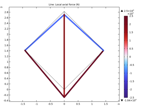
In the Settings window for Evaluation Group, type Axial Force in Members (2D) in the Label text field.
Global Evaluation 1
1
Right-click Axial Force in Members (2D) and choose Global Evaluation.
2
In the Settings window for Global Evaluation, locate the Expressions section.
3
4
In the Axial Force in Members (2D) toolbar, click  Evaluate.
The values in the evaluation group agree with those of the analytical reference solution.
Now create the 3D truss as a new model.
Add Component
In the Model Builder window, right-click the root node and choose Add Component>3D.
Add Physics
1
In the Home toolbar, click  Add Physics to open the Add Physics window.
2
Go to the Add Physics window.
3
In the tree, select Recently Used>Truss (truss).
4
Find the Physics interfaces in study subsection. In the table, clear the Solve check box for Study 1.
5
Click Add to Component 2 in the window toolbar.
6
In the Home toolbar, click  Add Physics to close the Add Physics window.
Add Study
1
In the Home toolbar, click  Add Study to open the Add Study window.
2
Go to the Add Study window.
3
Find the Studies subsection. In the Select Study tree, select General Studies>Stationary.
Switch off the 2D truss physics in this study.
4
Find the Physics interfaces in study subsection. In the table, clear the Solve check box for Truss (truss).
5
Click Add Study in the window toolbar.
6
In the Model Builder window, click the root node.
7
In the Home toolbar, click  Add Study to close the Add Study window.
Geometry 2
In the Model Builder window, under Component 2 (comp2) click Geometry 2.
Work Plane 1 (wp1)
1
In the Geometry toolbar, click  Work Plane.
2
In the Settings window for Work Plane, click  Show Work Plane.
Work Plane 1 (wp1)>Plane Geometry
In the Model Builder window, click Plane Geometry.
Work Plane 1 (wp1)>Square 1 (sq1)
1
In the Work Plane toolbar, click  Square.
2
In the Settings window for Square, locate the Size section.
3
In the Side length text field, type 2.
4
Locate the Rotation Angle section. In the Rotation text field, type 45.
5
Locate the Object Type section. From the Type list, choose Curve.
6
In the Work Plane toolbar, click  Build All.
Rotate 1 (rot1)
1
In the Model Builder window, right-click Geometry 2 and choose Transforms>Rotate.
2
In the Settings window for Rotate, locate the Input section.
3
Select the Keep input objects check box.
4
5
Locate the Rotation section. From the Axis type list, choose Cartesian.
6
In the y text field, type 1.
7
In the z text field, type 0.
8
In the Angle text field, type 90.
9
Click  Build All Objects.
Line Segment 1 (ls1)
1
In the Geometry toolbar, click  More Primitives and choose Line Segment.
2
In the Settings window for Line Segment, locate the Starting Point section.
3
From the Specify list, choose Coordinates.
4
Locate the Endpoint section. From the Specify list, choose Coordinates.
5
In the y text field, type sqrt(8).
6
Click  Build All Objects.
Definitions (comp2)
Add nonlocal average couplings for the members ac, ad, and cd and corresponding axial force variables.
Average 4 (aveop4)
1
In the Definitions toolbar, click  Nonlocal Couplings and choose Average.
2
In the Settings window for Average, type aveop_ac in the Operator name text field.
3
Locate the Source Selection section. From the Geometric entity level list, choose Edge.
4
Average 5 (aveop5)
1
In the Definitions toolbar, click  Nonlocal Couplings and choose Average.
2
In the Settings window for Average, type aveop_ad in the Operator name text field.
3
Locate the Source Selection section. From the Geometric entity level list, choose Edge.
4
Average 6 (aveop6)
1
In the Definitions toolbar, click  Nonlocal Couplings and choose Average.
2
In the Settings window for Average, type aveop_cd in the Operator name text field.
3
Locate the Source Selection section. From the Geometric entity level list, choose Edge.
4
Variables 2
1
In the Definitions toolbar, click  Local Variables.
2
In the Settings window for Variables, locate the Variables section.
3
Truss 2 (truss2)
Cross-Section Data 1
1
In the Model Builder window, under Component 2 (comp2)>Truss 2 (truss2) click Cross-Section Data 1.
2
In the Settings window for Cross-Section Data, locate the Cross-Section Data section.
3
In the A text field, type pi/4*0.05^2.
Cross-Section Data 2
1
In the Physics toolbar, click  Edges and choose Cross-Section Data.
2
3
In the Settings window for Cross-Section Data, locate the Cross-Section Data section.
4
In the A text field, type 2*pi/4*0.05^2.
Pinned 1
1
In the Physics toolbar, click  Points and choose Pinned.
2
Point Load 1
1
In the Physics toolbar, click  Points and choose Point Load.
2
3
In the Settings window for Point Load, locate the Force section.
4
Specify the FP vector as
Materials
Material Link 2 (matlnk2)
In the Model Builder window, under Component 2 (comp2) right-click Materials and choose More Materials>Material Link.
Study 2
In the Home toolbar, click  Compute.
Results
Force (truss2)
1
In the Settings window for 3D Plot Group, locate the Color Legend section.
2
Select the Show maximum and minimum values check box.
Proceed to compute the displacements at d (Vertex 2) and c (Vertex 5).
Displacement of Vertices (3D)
1
In the Model Builder window, right-click Displacement of Vertices (2D) and choose Duplicate.
2
In the Settings window for Evaluation Group, type Displacement of Vertices (3D) in the Label text field.
3
Locate the Data section. From the Dataset list, choose Study 2/Solution 2 (3) (sol2).
Point Evaluation 1
1
In the Model Builder window, expand the Displacement of Vertices (3D) node, then click Point Evaluation 1.
2
3
In the Settings window for Point Evaluation, locate the Expressions section.
4
5
In the Displacement of Vertices (3D) toolbar, click  Evaluate.
The results are nearly identical to those of the 2D case.
Finally, compute the axial force values.
Axial Force in Members (3D)
1
In the Model Builder window, right-click Axial Force in Members (2D) and choose Duplicate.
2
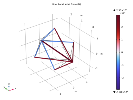
In the Settings window for Evaluation Group, type Axial Force in Members (3D) in the Label text field.
3
Locate the Data section. From the Dataset list, choose Study 2/Solution 2 (3) (sol2).
Global Evaluation 1
Because the applied force was doubled to get the same displacement as, in the 2D case, you need to divide the value of the axial force in member cd by 2 to get a value comparable to that of the 2D case.
1
In the Model Builder window, expand the Axial Force in Members (3D) node, then click Global Evaluation 1.
2
In the Settings window for Global Evaluation, locate the Expressions section.
3
4
In the Axial Force in Members (3D) toolbar, click  Evaluate.
Again, the values in the evaluation group agree very well with the reference solution.