Disc Brake Pad Wear

This example demonstrates how to compute wear of the friction material in a disc brake. Wear is modeled using a generalized form of the well-known Archard equation. The sliding velocity and the friction forces are computed from simple kinematic considerations. In addition, it is assumed that the disc has a much higher wear resistance than the pad, so that only wear of the friction material has to be considered. Thermal effects on the wear rate and thermal expansion are neglected.

Model Definition

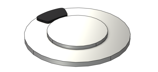
The simplified geometry of the disc and brake pad assembly is shown in Figure 1. Assuming a symmetric geometry, only half of the assembly needs to be modeled.

Figure 1: Disc brake geometry.

The entire assembly is considered to be linear elastic, and the brake disc is given material properties of steel. The material of the brake pad is assumed to have a stiffness that is one order or magnitude lower than that of the disc. All material properties are summarized in Table 1.

Table 1: Material Properties.
Property	Disc	Pad
Young’s modulus	210 GPa	10 GPa
Poisson's ratio	0.3	0.1
Density	7850 kg/m3	2000 kg/m3

The interaction between the disc and the pad is modeled using a contact condition. To ensure that the contact pressure is well resolved, the augmented Lagrangian method is used. The contact pressure is initiated by adding a boundary load to the top surface of the brake pad, and the effect of friction forces is accounted for by prescribing a relative slip velocity between the two parts. The angular velocity, ω, of the brake disc is assumed to be constant during the analysis. Since the origin of the global coordinate system is located in the center of the disc, the relative slip velocity, vslip, between the pad and the disc is given as

where r is the position vector to any point on the pad.

Wear involves a gradual removal of material at the surfaces in contact, and the process can be described with a rate equation. In this example, a generalized form of the Archard wear model is used, where the wear rate is given as

Here, hwear is the wear depth, kwear is a dimensionless wear constant, Tn is the contact pressure, Tn,ref is a reference pressure, n is a dimensionless exponent. By default, Tn,ref is set to 1 MPa and n to 1, which makes the above equation correspond to the classical form of the Archard wear equation.

Results and Discussion

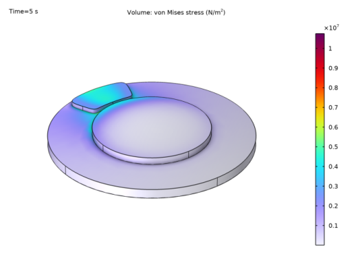
Figure 2 shows the distribution of the von Mises stress at the end of the simulation. At this point, material has been removed due to wear causing any initial peak in the stress to be smoothened out.

Figure 2: Distribution of von Mises stress in the pad and disc assembly.

If the contact between the pad and the disc was frictionless, the contact pressure would have a symmetric distribution over the pad surface. However, including friction forces results in a higher contact pressure at the leading edge of the brake pad compared to its trailing edge. This is shown in Figure 3 for the worn brake pad. As a result of the locally higher pressure, the wear rate, and subsequently the wear depth, is larger at the leading edge, see Figure 4. Due to the geometric changes resulting from the removal of material, the pressure distribution changes and the pressure peak at the leading edge eventually decreases over time.

Figure 3: Pressure distribution of the worn pad surface.

Figure 4: Distribution of the accumulated wear depth.

Notes About the COMSOL Implementation

The initial contact problem is solved in a first stationary study. By adding a subnode to the node, you can solve for dynamic friction forces even in a stationary study. To solve for the wear depth, add a second time-dependent study, and initialize the study with the values from the first study.

Wear is in this example modeled using the deformed geometry concept. This means that the geometry of the brake pad changes with time by using an adaptive meshing technique. Using this method to model wear thus also updates the contact conditions accordingly during the simulation.

Usually, wear problems require long time periods to generate any significant wear depths. One approach to avoid running long-term studies is to multiply the wear rate with an acceleration factor. The result may be interpreted as running the simulation for a time t times the wear acceleration factor, where t is the actual time period used in the simulation.

Structural_Mechanics_Module/Contact_and_Friction/disc_brake_wear

Modeling Instructions

From the menu, choose .

New

In the window, click

Model Wizard

In the window, click

In the tree, select .

Click .

Click

In the tree, select .

Click

Global Definitions

Parameters 1

In the window, under click .

In the window for , locate the section.

In the table, enter the following settings:


Name	Expression	Value	Description
v	60[km/h]	16.667 m/s	Vehicle speed
r_wheel	0.25[m]	0.25 m	Wheel radius
omega	v/r_wheel	66.667 1/s	Wheel angular velocity
wear_accel	100	100	Wear acceleration factor

Geometry 1

In the toolbar, click and choose .

Browse to the model’s Application Libraries folder and double-click the file disc_brake_geom_sequence.mph.

Form Assembly (fin)

In the window, under click .

In the window for , locate the section.

Select the check box.

From the list, choose .

In the toolbar, click

Definitions

Contact Pair 1 (ap1)

In the window, expand the node, then click .

In the window for , locate the section.

From the list, choose .

Cylindrical System 2 (sys2)

A boundary system is used to define the orientation of the relative slip velocity between the pad and the disc. In this case it is convenient to define the orientation of the boundary system axes based on cylindrical coordinates.

In the toolbar, click

and choose .

Boundary System 1 (sys1)

In the window, click .

In the window for , locate the section.

From the list, choose .

Find the subsection. From the list, choose .

From the list, choose .

Materials

Disc

In the window, under right-click and choose .

In the window for , type Disc in the text field.

Locate the section. In the list, select .

Click

Locate the section. In the table, enter the following settings:


Property	Variable	Value	Unit	Property group
Young’s modulus	E	210[GPa]	Pa	Young’s modulus and Poisson’s ratio
Poisson’s ratio	nu	0.3	1	Young’s modulus and Poisson’s ratio
Density	rho	7850[kg/m^3]	kg/m³	Basic

Click to expand the section. From the list, choose .

In the window toolbar, click

next to

, then choose .

In the window toolbar, click

next to

, then choose .

Pad

Right-click and choose .

Select Domain 3 only.

In the window for , type Pad in the text field.

Locate the section. In the table, enter the following settings:


Property	Variable	Value	Unit	Property group
Young’s modulus	E	10[GPa]	Pa	Young’s modulus and Poisson’s ratio
Poisson’s ratio	nu	0.1	1	Young’s modulus and Poisson’s ratio
Density	rho	2000	kg/m³	Basic

Click to expand the section. From the list, choose .

Solid Mechanics (solid)

Wear is a slow process and inertial effects can be neglected.

In the window, under click .

In the window for , locate the section.

From the list, choose .

Fixed Constraint 1

In the toolbar, click

and choose .

Select Boundary 8 only.

Symmetry 1

In the toolbar, click

and choose .

Select Boundary 3 only.

Prescribed Displacement 1

In the toolbar, click

and choose .

In the window for , locate the section.

Select the check box.

Select Boundary 16 only.

Boundary Load 1

In the toolbar, click

and choose .

Select Boundary 16 only.

In the window for , locate the section.

From the list, choose .

Specify the Ftot vector as


0	x
0	y
-10[kN]	z

Contact 1

In the window, click .

In the window for , locate the section.

From the list, choose .

Locate the section. From the list, choose .

Locate the section. In the Tn text field, type 5e6.

Slip Velocity 1

In the toolbar, click

and choose .

In the window for , locate the section.

In the μ text field, type 0.45.

Locate the section. Specify the vslip vector as


omega*sys2.r	t1
0	t2

The input is given in the boundary system selected in the section.

Click the

button in the toolbar.

In the dialog box, in the tree, select the check box for the node .

Click .

In the window for , click to expand the section.

Select the check box.

Contact 1

In the window, click .

Wear 1

In the toolbar, click

and choose .

In the window for , locate the section.

In the kwear text field, type 1e-14*wear_accel.

The factor wear_accel artificially accelerates the wear rate in order to reduce the computation time. In this case wear_accel is set to 100 and the time-dependent solver spans an interval of only 5 s. Alternatively, this model could be run with no acceleration factor but over a time span of 500 s. This would yield practically identical results, though at the cost of a significantly higher computation time.

Mesh 1

Free Triangular 1

In the toolbar, click