|
|
|
|
1
|
|
2
|
In the Select Physics tree, select Structural Mechanics>Electromagnetics-Structure Interaction>Magnetomechanics>Magnetomechanics.
|
|
3
|
Click Add.
|
|
4
|
Click
|
|
5
|
|
6
|
Click
|
|
1
|
|
2
|
|
1
|
|
2
|
|
3
|
|
1
|
|
2
|
|
3
|
|
4
|
|
1
|
|
2
|
|
3
|
|
4
|
|
5
|
|
1
|
|
2
|
|
3
|
|
4
|
|
5
|
|
6
|
|
1
|
|
2
|
|
3
|
|
4
|
|
5
|
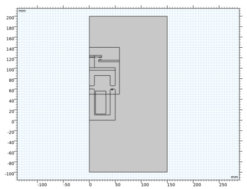
Select the object r3 only.
|
|
1
|
|
2
|
Select the object dif1 only.
|
|
1
|
|
2
|
|
3
|
|
4
|
|
5
|
|
6
|
|
1
|
|
2
|
|
3
|
|
4
|
|
5
|
|
1
|
|
2
|
|
3
|
|
4
|
|
5
|
|
1
|
|
2
|
|
3
|
|
4
|
|
5
|
|
6
|
|
7
|
|
1
|
|
2
|
|
3
|
|
4
|
|
5
|
|
1
|
|
2
|
|
3
|
|
4
|
|
5
|
|
1
|
|
2
|
|
3
|
|
4
|
|
5
|
|
6
|
|
1
|
|
2
|
|
3
|
|
4
|
|
1
|
|
2
|
|
3
|
|
4
|
|
1
|
|
2
|
|
3
|
|
4
|
|
1
|
|
2
|
|
3
|
|
4
|
On the object mov2(7), select Points 3, 5, and 7 only.
|
|
5
|
|
1
|
|
2
|
|
3
|
|
4
|
On the object mov2(3), select Points 1 and 2 only.
|
|
5
|
|
1
|
|
2
|
|
3
|
|
4
|
|
5
|
|
1
|
|
2
|
|
3
|
|
4
|
|
5
|
|
6
|
|
7
|
|
8
|
|
9
|
|
10
|
|
1
|
|
2
|
On the object r12, select Boundary 5 only.
|
|
1
|
|
2
|
|
3
|
|
4
|
|
5
|
|
6
|
|
1
|
|
3
|
|
4
|
|
6
|
|
7
|
|
1
|
|
3
|
|
4
|
|
6
|
|
7
|
|
1
|
|
1
|
|
1
|
|
2
|
|
3
|
In the tree, select Built-in>Air.
|
|
4
|
|
5
|
|
6
|
|
1
|
In the Model Builder window, under Component 1 (comp1)>Materials click Soft Iron (Without Losses) (mat2).
|
|
1
|
|
2
|
In the tree, select Built-in>Copper.
|
|
3
|
|
1
|
|
1
|
|
2
|
|
3
|
|
1
|
|
1
|
|
2
|
In the tree, select Built-in>Aluminum.
|
|
3
|
|
4
|
|
1
|
|
2
|
|
3
|
|
1
|
|
1
|
|
3
|
|
4
|
|
5
|
|
6
|
Click to expand the Viscous Damping section. From the Damping type list, choose Total damping constant.
|
|
7
|
|
1
|
|
1
|
|
1
|
|
1
|
|
2
|
|
3
|
|
4
|
|
5
|
|
6
|
|
1
|
|
1
|
|
2
|
In the Settings window for Contact, click to expand the Contact Surface Offset and Adjustment section.
|
|
3
|
|
1
|
|
2
|
|
3
|
|
1
|
|
2
|
|
4
|
|
5
|
|
1
|
|
2
|
|
1
|
|
2
|
|
4
|
|
5
|
|
6
|
|
7
|
|
8
|
|
9
|
|
1
|
|
2
|
|
4
|
|
5
|
|
1
|
|
1
|
|
1
|
In the Model Builder window, under Component 1 (comp1)>Multiphysics click Magnetomechanical Forces 1 (mmf1).
|
|
1
|
|
2
|
|
1
|
|
2
|
|
1
|
|
2
|
|
3
|
|
5
|
|
6
|
|
7
|
|
1
|
|
2
|
|
3
|
|
5
|
|
6
|
|
1
|
|
2
|
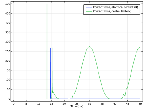
In the Settings window for Global Variable Probe, type Contact force, electrical contact in the Label text field.
|
|
3
|
|
4
|
Locate the Expression section. In the Expression text field, type solid.dcnt1.T_toty_p1*(solid.dcnt1.T_toty_p1<500[N])+500[N]*(solid.dcnt1.T_toty_p1>500[N]).
|
|
5
|
Select the Description check box. In the associated text field, type Contact force, electrical contact.
|
|
6
|
|
1
|
|
2
|
In the Settings window for Global Variable Probe, type Contact force, central limb in the Label text field.
|
|
3
|
|
4
|
|
5
|
In the Expression text field, type solid.dcnt1.T_toty_p2*(solid.dcnt1.T_toty_p2<500[N])+500[N]*(solid.dcnt1.T_toty_p2>500[N]).
|
|
1
|
|
1
|
|
2
|
|
3
|
|
4
|
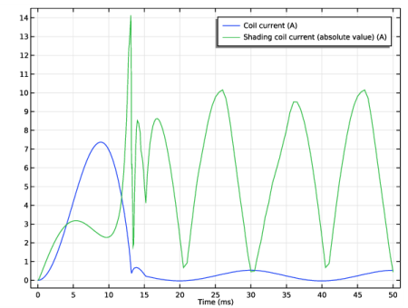
Click Replace Expression in the upper-right corner of the Expression section. From the menu, choose Component 1 (comp1)>Magnetic Fields>Coil parameters>mf.ICoil_1 - Coil current - A.
|
|
5
|
|
1
|
|
2
|
In the Settings window for Global Variable Probe, type I_shading_coil in the Variable name text field.
|
|
3
|
|
4
|
|
5
|
Select the Description check box. In the associated text field, type Shading coil current (absolute value).
|
|
1
|
|
2
|
|
3
|
|
4
|
|
5
|
|
6
|
|
1
|
|
2
|
|
3
|
|
4
|
|
1
|
|
2
|
|
3
|
|
1
|
|
2
|
|
3
|
|
4
|
|
5
|
|
6
|
|
1
|
|
2
|
|
3
|
|
4
|
|
1
|
In the Model Builder window, expand the Study 1>Solver Configurations node, then click Study 1>Step 1: Time Dependent.
|
|
2
|
|
3
|
Select the Plot check box.
|
|
4
|
|
5
|
|
1
|
|
2
|
|
1
|
|
2
|
|
3
|
|
1
|
|
2
|
|
1
|
|
2
|
|
1
|
|
2
|
In the Settings window for Force Calculation, type Force Calculation, for Postprocessing in the Label text field.
|
|
1
|
|
2
|
|
3
|
|
1
|
|
2
|
|
4
|
|
1
|
|
2
|
In the Settings window for 1D Plot Group, type Contact Force, Electrical Contact in the Label text field.
|
|
3
|
|
4
|
|
5
|
|
6
|
|
1
|
|
2
|
In the Settings window for Global, click Replace Expression in the upper-right corner of the y-Axis Data section. From the menu, choose Component 1 (comp1)>Definitions>T_toty_p1 - Contact force, electrical contact - N.
|
|
3
|