|
|
|


|
1
|
|
2
|
In the Application Libraries window, select Structural Mechanics Module>Tutorials>bracket_basic in the tree.
|
|
3
|
Click
|
|
1
|
|
2
|
|
3
|
Find the Studies subsection. In the Select Study tree, select Preset Studies for Selected Physics Interfaces>Random Vibration (PSD).
|
|
4
|
|
5
|
|
1
|
|
2
|
|
3
|
|
4
|
|
5
|
|
6
|
|
7
|
|
1
|
|
2
|
|
3
|
|
4
|
In the tree, select Component 1 (Comp1)>Solid Mechanics (Solid)>Linear Elastic Material 1>Damping 1.
|
|
5
|
Right-click and choose Disable.
|
|
1
|
In the Model Builder window, expand the Global Definitions>Reduced-Order Modeling node, then click Global Reduced Model Inputs 1.
|
|
2
|
|
1
|
|
2
|
|
3
|
|
4
|
|
5
|
|
6
|
|
7
|
|
8
|
In the Settings window for Rigid Connector, locate the Prescribed Displacement at Center of Rotation section.
|
|
9
|
|
10
|
|
11
|
|
12
|
|
13
|
|
1
|
|
2
|
|
3
|
Specify the F vector as
|
|
1
|
In the Model Builder window, under Component 1 (comp1) right-click Definitions and choose Variables.
|
|
2
|
|
1
|
In the Model Builder window, expand the Step 1: Model Reduction node, then click Frequency Domain 1.
|
|
2
|
|
3
|
|
1
|
Click
|
|
1
|
|
2
|
|
3
|
|
4
|
Browse to the model’s Application Libraries folder and double-click the file bracket_random_vibration_log.txt.
|
|
1
|
|
2
|
|
3
|
|
4
|
Find the Intervals subsection. In the table, enter the following settings:
|
|
5
|
|
6
|
|
1
|
|
2
|
|
3
|
Find the Intervals subsection. In the table, enter the following settings:
|
|
1
|
In the Model Builder window, under Global Definitions>Reduced-Order Modeling click Random Vibration 1 (rvib1).
|
|
2
|
|
3
|
|
5
|
|
6
|
|
1
|
|
2
|
|
4
|
Locate the Expressions section. In the table, enter the following settings:
|
|
5
|
|
6
|
Click
|
|
1
|
Go to the Table window.
|
|
2
|
|
1
|
|
2
|
|
3
|
|
4
|
|
5
|
|
6
|
|
1
|
|
2
|
|
3
|
|
1
|
|
2
|
|
4
|
Locate the Expressions section. In the table, enter the following settings:
|
|
5
|
|
6
|
Click
|
|
1
|
Go to the Table window.
|
|
2
|
|
1
|
|
2
|
|
3
|
|
4
|
|
1
|
|
2
|
|
3
|
|
1
|
|
2
|
|
4
|
Locate the Expressions section. In the table, enter the following settings:
|
|
5
|
|
6
|
|
1
|
Go to the Table window.
|
|
2
|
|
1
|
|
2
|
|
3
|
|
1
|
|
2
|
|
3
|
|
4
|
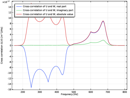
In the associated text field, type Frequnecy [Hz].
|
|
5
|
|
6
|
In the associated text field, type Cross correlation (U,V) [m^2/Hz].
|
|
7
|
|
8
|
|
1
|
|
2
|
|
3
|
|
1
|
|
2
|
|
3
|
|
4
|
Select the Description check box.
|
|
5
|
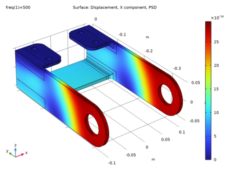
In the associated text field, type Displacement, X component, PSD.
|
|
6
|
|
7
|
|
1
|
|
2
|
|
3
|
|
1
|
|
2
|
|
3
|
|
4
|
|
5
|
|
6
|
|
7
|
|
8
|
|
9
|
|
1
|
|
2
|
|
3
|
|
4
|
|
1
|
|
2
|
|
3
|
|
4
|
|
5
|
|
1
|
|
2
|
|
3
|
|
4
|
|
1
|
|
2
|
|
3
|
|
4
|
|
5
|
|
1
|
|
2
|
|
3
|
|
1
|
|
2
|
|
3
|
|
4
|
Select the Description check box.
|
|
5
|
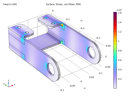
In the associated text field, type Stress, von Mises, RMS.
|
|
6
|
|
7
|
|
1
|
|
2
|
|
1
|
|
2
|
|
3
|
|
4
|
Select the Description check box.
|
|
5
|
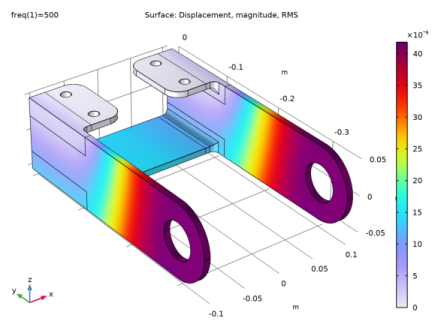
In the associated text field, type Displacement, magnitude, RMS.
|
|
6
|
|
1
|
|
2
|
|
1
|
|
2
|
|
3
|
|
4
|
Select the Description check box.
|
|
5
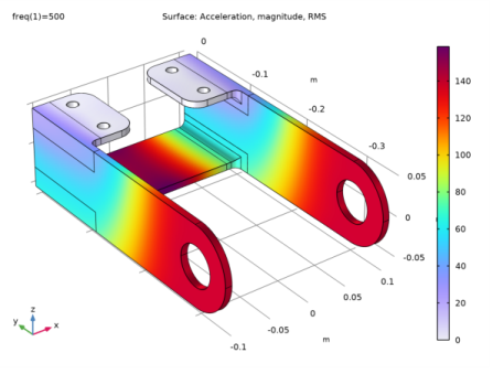
|
In the associated text field, type Acceleration, magnitude, RMS.
|
|
6
|