
|
|
|

|
1
|
|
2
|
In the Application Libraries window, select Structural Mechanics Module>Tutorials>bracket_basic in the tree.
|
|
3
|
Click
|
|
1
|
|
2
|
|
1
|
|
2
|
|
3
|
|
4
|
|
5
|
Locate the Units section. In the table, enter the following settings:
|
|
6
|
|
1
|
|
2
|
|
3
|
|
1
|
In the Model Builder window, under Component 1 (comp1) right-click Solid Mechanics (solid) and choose Boundary Load.
|
|
2
|
|
3
|
|
4
|
Locate the Coordinate System Selection section. From the Coordinate system list, choose Boundary System 1 (sys1).
|
|
5
|
|
1
|
|
2
|
|
3
|
Find the Studies subsection. In the Select Study tree, select Preset Studies for Selected Physics Interfaces>Linear Buckling.
|
|
4
|
|
5
|
|
1
|
|
1
|
|
2
|
|
3
|
|
5
|
Locate the Expressions section. In the table, enter the following settings:
|
|
6
|
Click
|
|
1
|
|
2
|
|
3
|
|
1
|
|
2
|
|
3
|
|
4
|
|
5
|
|
1
|
|
2
|
|
3
|
|
4
|
Click
|
|
1
|
|
2
|
|
3
|
In the Model Builder window, expand the Study 2>Solver Configurations>Solution 3 (sol3)>Stationary Solver 1 node.
|
|
4
|
Right-click Study 2>Solver Configurations>Solution 3 (sol3)>Stationary Solver 1>Parametric 1 and choose Stop Condition.
|
|
5
|
|
6
|
Click
|
|
8
|
|
9
|
|
10
|
|
1
|
|
2
|
|
3
|
|
1
|
|
3
|
|
4
|
|
5
|
|
1
|
|
2
|
|
3
|
|
4
|
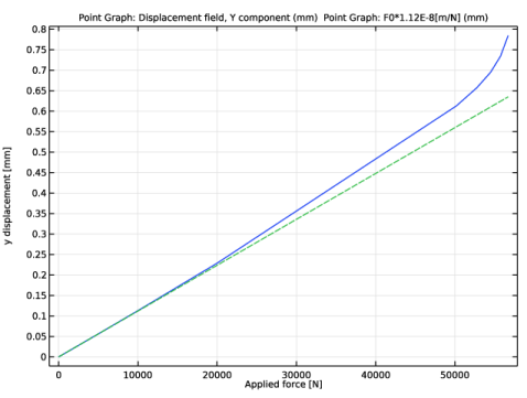
In the associated text field, type Applied force [N].
|
|
5
|
|
6
|
In the associated text field, type y displacement [mm].
|
|
1
|
|
3
|
|
4
|
|
5
|
|
6
|
Click to expand the Coloring and Style section. Find the Line style subsection. From the Line list, choose Dashed.
|
|
7
|