|
|
|


|
1
|
|
2
|
In the Application Libraries window, select Structural Mechanics Module>Tutorials>bracket_basic in the tree.
|
|
3
|
Click
|
|
1
|
|
2
|
|
1
|
|
2
|
|
4
|
|
5
|
In the Function table, enter the following settings:
|
|
1
|
|
2
|
|
3
|
|
4
|
|
5
|
|
6
|
Locate the Units section. In the table, enter the following settings:
|
|
7
|
|
8
|
|
9
|
Click
|
|
1
|
|
2
|
|
3
|
|
4
|
|
1
|
|
2
|
|
3
|
|
4
|
|
5
|
|
1
|
In the Model Builder window, under Component 2 (comp2)>Global ODEs and DAEs (ge) click Global Equations 1.
|
|
2
|
|
4
|
|
5
|
|
6
|
Click
|
|
7
|
|
8
|
Click OK.
|
|
9
|
|
10
|
|
11
|
|
12
|
Click OK.
|
|
1
|
|
2
|
|
3
|
|
4
|
|
5
|
|
6
|
|
1
|
In the Settings window for Study, type Study 1: Fourier Coefficient Generation in the Label text field.
|
|
2
|
|
1
|
In the Model Builder window, under Study 1: Fourier Coefficient Generation click Step 1: Time Dependent.
|
|
2
|
|
3
|
|
4
|
Locate the Physics and Variables Selection section. In the table, clear the Solve for check box for Solid Mechanics (solid).
|
|
1
|
|
2
|
|
3
|
|
4
|
|
5
|
Locate the Physics and Variables Selection section. In the table, clear the Solve for check box for Solid Mechanics (solid).
|
|
1
|
|
2
|
|
1
|
In the Model Builder window, expand the Study 1: Fourier Coefficient Generation>Solver Configurations>Solution 1 (sol1) node.
|
|
2
|
|
3
|
|
4
|
|
5
|
|
1
|
|
2
|
|
3
|
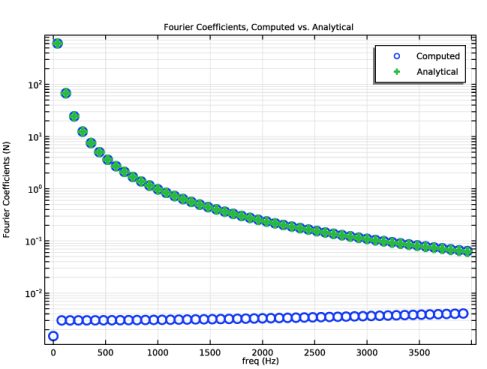
In the Settings window for 1D Plot Group, type Fourier Coefficients, Computed vs. Analytical in the Label text field.
|
|
4
|
|
5
|
|
6
|
|
7
|
|
8
|
In the associated text field, type freq (Hz).
|
|
9
|
|
10
|
In the associated text field, type Fourier Coefficients (N).
|
|
11
|
|
1
|
|
2
|
|
4
|
Click to expand the Coloring and Style section. Find the Line style subsection. From the Line list, choose None.
|
|
5
|
|
6
|
|
7
|
|
8
|
|
1
|
|
2
|
|
4
|
Locate the Data section. From the Dataset list, choose Study 1: Fourier Coefficient Generation/Solution 1 (sol1).
|
|
5
|
|
6
|
|
7
|
Locate the Coloring and Style section. Find the Line markers subsection. From the Marker list, choose Plus sign.
|
|
8
|
Locate the Legends section. In the table, enter the following settings:
|
|
9
|
|
1
|
|
2
|
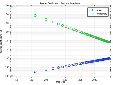
In the Settings window for 1D Plot Group, type Fourier Coefficients; Real and Imaginary in the Label text field.
|
|
3
|
|
4
|
|
5
|
|
6
|
|
7
|
|
8
|
|
9
|
In the associated text field, type freq (Hz).
|
|
10
|
|
11
|
In the associated text field, type Fourier Coefficients (N).
|
|
1
|
|
2
|
|
4
|
Locate the Coloring and Style section. Find the Line style subsection. From the Line list, choose None.
|
|
5
|
|
6
|
|
7
|
|
8
|
|
10
|
|
1
|
|
2
|
|
3
|
|
4
|
|
5
|
|
6
|
|
7
|
|
1
|
|
2
|
|
3
|
|
4
|
|
5
|
|
6
|
|
1
|
|
2
|
|
3
|
Find the Studies subsection. In the Select Study tree, select Preset Studies for Selected Physics Interfaces>Solid Mechanics>Frequency Domain, Modal.
|
|
4
|
|
5
|
|
1
|
In the Model Builder window, under Study 2: Frequency Domain Modal + FFT click Step 1: Eigenfrequency.
|
|
2
|
|
3
|
|
5
|
Locate the Physics and Variables Selection section. Select the Modify model configuration for study step check box.
|
|
6
|
In the tree, select Component 1 (Comp1)>Solid Mechanics (Solid)>Linear Elastic Material 1>Damping 1.
|
|
7
|
Right-click and choose Disable.
|
|
8
|
|
9
|
|
1
|
|
2
|
|
3
|
|
4
|
Locate the Physics and Variables Selection section. Select the Modify model configuration for study step check box.
|
|
5
|
|
6
|
|
1
|
|
2
|
|
3
|
|
4
|
|
5
|
Locate the Physics and Variables Selection section. Select the Modify model configuration for study step check box.
|
|
6
|
|
7
|
|
8
|
|
1
|
|
2
|
|
3
|
|
4
|
|
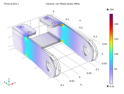
1
|
In the Model Builder window, expand the Stress: Frequency Domain Modal + FFT node, then click Volume 1.
|
|
2
|
|
3
|
|
4
|
|
1
|
|
2
|
In the Settings window for 1D Plot Group, type Displacement Amplitude [Frequency Response] in the Label text field.
|
|
3
|
|
4
|
Locate the Data section. From the Dataset list, choose Study 2: Frequency Domain Modal + FFT/Solution Store 3 (sol5).
|
|
5
|
|
6
|
|
1
|
|
3
|
In the Settings window for Point Graph, click Replace Expression in the upper-right corner of the y-Axis Data section. From the menu, choose Component 1 (comp1)>Solid Mechanics>Displacement>Displacement amplitude (material and geometry frames) - m>solid.uAmpX - Displacement amplitude, X component.
|
|
4
|
|
5
|
Click to expand the Coloring and Style section. Find the Line style subsection. From the Line list, choose None.
|
|
6
|
|
7
|
|
8
|
|
1
|
|
2
|
In the Settings window for Boundary Load, type Boundary Load, Time Domain Amplitude in the Label text field.
|
|
3
|
|
4
|
|
5
|
|
1
|
In the Model Builder window, under Study 2: Frequency Domain Modal + FFT click Step 2: Frequency Domain, Modal.
|
|
2
|
In the Settings window for Frequency Domain, Modal, locate the Physics and Variables Selection section.
|
|
3
|
In the tree, select Component 1 (Comp1)>Solid Mechanics (Solid)>Boundary Load, Time Domain Amplitude.
|
|
4
|
Right-click and choose Disable.
|
|
1
|
|
2
|
In the Settings window for Frequency to Time FFT, locate the Physics and Variables Selection section.
|
|
3
|
In the tree, select Component 1 (Comp1)>Solid Mechanics (Solid)>Boundary Load, Time Domain Amplitude.
|
|
4
|
Right-click and choose Disable.
|
|
1
|
|
2
|
|
3
|
Find the Studies subsection. In the Select Study tree, select Preset Studies for Selected Physics Interfaces>Solid Mechanics>Time Dependent, Modal.
|
|
4
|
|
5
|
|
1
|
In the Settings window for Study, type Study 3: Time-Dependent Modal [Verification] in the Label text field.
|
|
1
|
In the Model Builder window, under Study 3: Time-Dependent Modal [Verification] click Step 1: Time Dependent, Modal.
|
|
2
|
|
3
|
|
4
|
Locate the Physics and Variables Selection section. Select the Modify model configuration for study step check box.
|
|
5
|
|
6
|
Right-click and choose Disable.
|
|
7
|
|
8
|
|
1
|
|
2
|
|
3
|
|
4
|
|
5
|
|
6
|
|
7
|
|
8
|
|
9
|
|
1
|
|
2
|
|
3
|
|
4
|
|
1
|
|
2
|
|
3
|
|
4
|
|
1
|
|
2
|
|
1
|
|
2
|
|
3
|
|
4
|
|
5
|
|
1
|
|
3
|
|
4
|
|
5
|
|
6
|
|
7
|
|
8
|
|
1
|
|
2
|
|
3
|
|
4
|
|
5
|
|
6
|
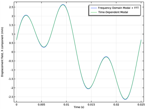
Locate the Legends section. In the table, enter the following settings:
|
|
7
|
|
1
|
|
2
|
|
1
|
|
2
|
|
3
|
|
4
|
|
6
|
|
7
|
|
1
|
|
2
|
|
3
|
|
4
|
|
6
|
|
7
|
|
8
|