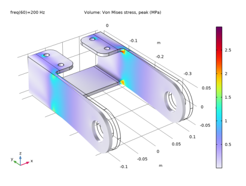
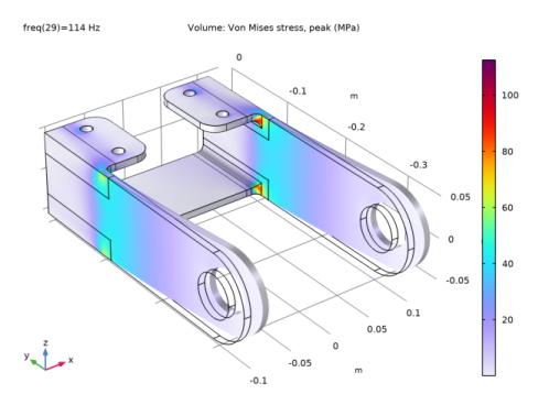
|
|
|
|
1
|
|
2
|
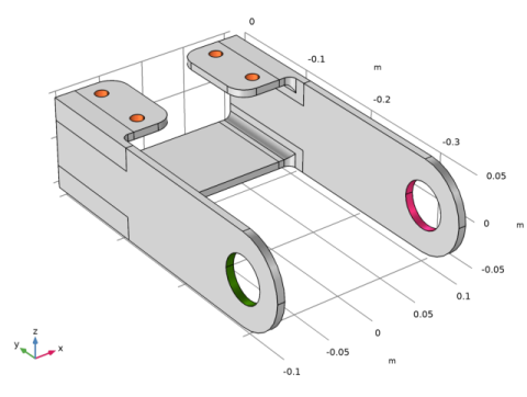
In the Application Libraries window, select Structural Mechanics Module>Tutorials>bracket_basic in the tree.
|
|
3
|
Click
|
|
1
|
|
2
|
|
3
|
|
1
|
In the Model Builder window, expand the Component 1 (comp1)>Materials node, then click Structural steel (mat1).
|
|
2
|
|
1
|
|
2
|
|
4
|
|
5
|
|
1
|
|
2
|
|
3
|
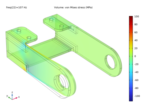
Find the Studies subsection. In the Select Study tree, select Preset Studies for Selected Physics Interfaces>Frequency Domain, Modal.
|
|
4
|
|
5
|
|
1
|
|
2
|
|
1
|
|
2
|
|
3
|
|
4
|
|
1
|
|
1
|
|
2
|
|
3
|
|
4
|
In the associated text field, type Frequency (Hz).
|
|
1
|
|
3
|
|
4
|
|
5
|
|
6
|
|
7
|
|
8
|
|
9
|
|
1
|
|
2
|
|
3
|
|
1
|
|
3
|
|
4
|
|
5
|
|
6
|
|
7
|
|
8
|
|
9
|
|
11
|
|
1
|
|
2
|
|
3
|
|
4
|
|
5
|
|
6
|
|
1
|
|
2
|
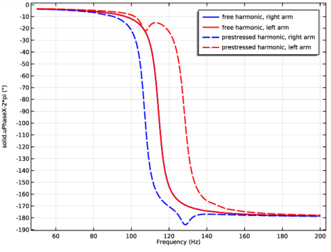
In the Settings window for 1D Plot Group, type Displacement phase, X component in the Label text field.
|
|
3
|
|
4
|
|
5
|
In the associated text field, type Frequency (Hz).
|
|
1
|
|
2
|
|
3
|
|
4
|
Click Replace Expression in the upper-right corner of the y-Axis Data section. From the menu, choose Component 1 (comp1)>Solid Mechanics>Displacement>Displacement phase (material and geometry frames) - rad>solid.uPhaseX - Displacement phase, X component.
|
|
5
|
|
6
|
|
7
|
|
9
|
|
1
|
|
2
|
|
3
|
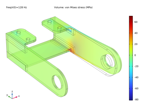
Find the Studies subsection. In the Select Study tree, select Preset Studies for Selected Physics Interfaces>Frequency Domain, Prestressed.
|
|
4
|
|
5
|
|
1
|
|
2
|
|
1
|
|
2
|
|
3
|
|
4
|
|
5
|
Locate the Units section. In the table, enter the following settings:
|
|
6
|
|
1
|
|
2
|
|
3
|
|
4
|
Locate the Coordinate System Selection section. From the Coordinate system list, choose Boundary System 1 (sys1).
|
|
5
|
|
1
|
|
2
|
|
3
|
|
1
|
|
2
|
|
3
|
|
4
|
|
1
|
|
1
|
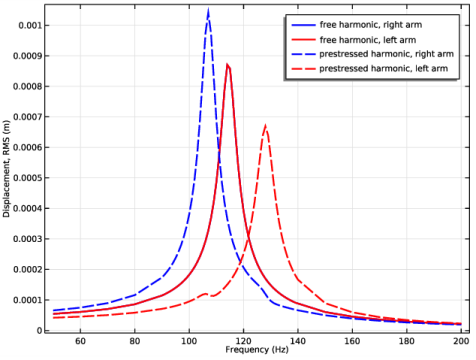
In the Model Builder window, under Results>Displacement, RMS, Ctrl-click to select Point Graph 1 and Point Graph 2.
|
|
2
|
Right-click and choose Duplicate.
|
|
1
|
|
2
|
|
3
|
Locate the Coloring and Style section. Find the Line style subsection. From the Line list, choose Dashed.
|
|
4
|
|
5
|
Locate the Legends section. In the table, enter the following settings:
|
|
1
|
|
2
|
|
3
|
|
4
|
Locate the Coloring and Style section. Find the Line style subsection. From the Line list, choose Dashed.
|
|
5
|
|
6
|
Locate the Legends section. In the table, enter the following settings:
|
|
7
|
|
1
|
In the Model Builder window, under Results>Datasets right-click Cut Point 3D 1 and choose Duplicate.
|
|
2
|
|
3
|
|
1
|
In the Model Builder window, under Results>Displacement phase, X component right-click Point Graph 1 and choose Duplicate.
|
|
2
|
|
3
|
|
4
|
|
5
|
Locate the Legends section. In the table, enter the following settings:
|
|
6
|
|
1
|
|
2
|