PDF

k·p Method for Strained Wurtzite GaN Band Structure
This benchmark model computes the valence band structure of an unstrained and a strained bulk GaN wurtzite crystal, as a tutorial for users who wish to set up multiple wave-function components with the Schrödinger Equation interface. The model follows the formulation given in the reference paper by Chuang and Chang (Ref. 1). The diagonal and off-diagonal elements of the Hamiltonian matrix are entered using built-in features, with detailed instructions in the model documentation. The computed eigenvalues agree well with the analytic solution and Fig. 5 in the paper.
Introduction
For the Schrödinger Equation physics interface, if the wave function has more than one component, then the Hamiltonian becomes a matrix. The number of elements of the matrix grows as the square of the number of wave-function components. Each element can include several terms of zero, one, or two partial derivatives. A number of built-in features have been created to provide flexible and efficient ways to enter these terms into the graphical user interface within limited window size.
Because the main purpose of this model is to illustrate the usage of these built-in features, a particularly simple system of bulk GaN crystal is chosen for clarity. Specifically, the model uses the upper left 3-by-3 matrix of the block-diagonalized 6-by-6 Hamiltonian for the demonstration. Once you have understood the procedure for setting up this simple Hamiltonian matrix, you should be able to build your own models of higher complexity.
An additional benefit of this simple system is that an analytic formula for the matrix elements exists and the result from the solution of the Schrödinger Equation can be compared against the eigenvalues of the 3-by-3 matrix equation with analytic coefficients.
Model Definition
Gallium nitride (GaN) is an important wideband-gap semiconductor material for optoelectronics, high-power, and high-frequency applications. Chuang and Chang published their derivation and computation of the 6-by-6 Hamiltonian matrix for wurtzite crystals including GaN in 1996 (Ref. 1). In Eq. (45) of the paper, the 6-by-6 Hamiltonian matrix is block diagonalized, and the upper left 3-by-3 matrix reads
(1)
The matrix elements are given by Eqs. (34) and (42) in Ref. 1. To compare with Fig. 5 in the paper, set the crystal momentum ky to zero. For the Schrödinger Equation interface, kx and kz are replaced by the partial derivatives i∂/∂x and i∂/∂z, respectively. Note that there is no minus sign in front of the imaginary unit i because of the engineering sign convention adopted by all COMSOL physics interfaces: a plane wave is exp(−ikx + iωt), not exp(ikx − iωt).
As an example of entering the matrix elements into the graphical user interface, consider the element F at the (1,1) position of the 3-by-3 Hamiltonian matrix. Eq. (34) in the paper gives
(2)
(3)
(4)
(5)
(6)
In Equation 3 and Equation 4, the partial derivative on the left side is understood to operate on both the Ai coefficient and the wave function (not explicitly displayed on the right end). In general, the Ai coefficients and other material parameters can be spatially varying, for example, in heterostructures or quantum dots. Here, for the simple case of a bulk crystal, all of these parameters are constants.
The first terms in Equation 3 and Equation 4 involve second-order derivatives, while the last terms λε and θε are strain-dependent constants given by the formulas Equation 5 and Equation 6. The built-in features Second Order Hamiltonian and Zeroth Order Hamiltonian (or Electron Potential Energy for diagonal elements) will be used to enter each type of terms in the model, respectively, as detailed in the Modeling Instructions section.
Since the model solves for the bulk crystal, it suffices to create a small square domain (smaller than the smallest wavelength of interest), and use the Floquet-Bloch periodic boundary conditions. In this case, a small number of mesh elements is enough.
For the analytic solution, a global equation is used to set up the 3-by-3 matrix equation. The All option of the Eigenvalue search method is used to obtain all 3 eigenvalues.
Results and Discussion
Figure 1 and Figure 2 show the computed unstrained and strained heavy hole (HH), light hole (LH), and crystal-field split-off hole (CH) dispersions along the positive x-axis and negative z-axis directions, agreeing well with analytic solution (circles) and Fig. 5 in Ref. 1.
Figure 1: Unstrained valence band structure of bulk GaN wurtzite crystal.
Figure 2: Strained valence band structure of bulk GaN wurtzite crystal.
Figure 3 compares the 2D band energy surfaces along the x and z directions for the 3 valence bands between computed values (color surface) and analytic solution (gray wireframe). The agreement is very good.
Figure 3: Strained valence band structure of bulk GaN wurtzite crystal.
Reference
1. S.L. Chuang and C.S. Chang, “k·p method for strained wurtzite semiconductors,” Phys. Rev. B, vol. 54, p. 2491, 1996.
Application Library path: Semiconductor_Module/Verification_Examples/k_dot_p_method_strained_wurtzite_gan_band_structure
Modeling Instructions
From the File menu, choose New.
New
In the New window, click  Model Wizard.
Model Wizard
1
In the Model Wizard window, click  2D.
2
In the Select Physics tree, select Semiconductor>Schrödinger Equation (schr).
3
Click Add.
Since there are 3 valence bands of interest, set the number of wave function components to 3.
4
In the Number of wave function components text field, type 3.
5
Click  Study.
6
In the Select Study tree, select Preset Studies for Selected Physics Interfaces>Eigenvalue.
7
Geometry 1
The Model Wizard ended at the Settings pane for the Geometry node in the Model Builder tree structure. We can use this opportunity to select a convenient length unit.
1
In the Model Builder window, under Component 1 (comp1) click Geometry 1.
2
In the Settings window for Geometry, locate the Units section.
3
From the Length unit list, choose Å.
The geometry can be a simple square for setting up the Floquet-Bloch boundary conditions. The size of the domain should be smaller than the shortest wavelength, to prevent spurious modes (a related mechanical model is thin_film_baw_resonator_dispersion_diagram in the MEMS Module, where a narrow domain is used).
Square 1 (sq1)
1
In the Geometry toolbar, click  Square.
2
In the Settings window for Square, click  Build All Objects.
In this 2D model we will look at the valence band dispersion along the x and z directions. Change the default second axis name from y to z for clarity.
Component 1 (comp1)
1
In the Model Builder window, click Component 1 (comp1).
2
In the Settings window for Component, locate the Frames section.
3
Find the Spatial frame coordinates subsection. In the table, enter the following settings:
4
Find the Material frame coordinates subsection. In the table, enter the following settings:
Enter the GaN material parameters as listed in Table III of Chuang and Chang’s paper. Only the valence band parameters are needed for this model. First enter the energy parameters Δ1, Δso, Δ2, Δ3, and Δ.
Global Definitions
Parameters 1 - GaN
1
In the Model Builder window, under Global Definitions click Parameters 1.
2
In the Settings window for Parameters, type Parameters 1 - GaN in the Label text field.
3
Locate the Parameters section. In the table, enter the following settings:
Next enter the valence band effective-mass parameters A1 ~ A6.
4
Next enter the deformation potentials D1 ~ D4.
5
Next enter the elastic stiffness constants C13 and C33.
6
Finally to prevent too long a list of parameters when setting up sweeps, exclude these parameters from the selection list.
7
Click to expand the Visibility section. Clear the Show in parameter selections check box.
Now set up the swept parameters.
Parameters 2 - Sweeps
1
In the Home toolbar, click  Parameters and choose Add>Parameters.
2
In the Settings window for Parameters, type Parameters 2 - Sweeps in the Label text field.
3
Locate the Parameters section. In the table, enter the following settings:
To conveniently create a plot to compare with Fig. 5 in the paper, set up a swept parameter kp such that its positive axis represents the kx axis and the negative axis represents the kz axis.
4
For comparing with analytic solutions, enter the formulas from Eq. (34) and Eq. (42) in the paper. These parameters also are not needed to be in the selection list. In these formulas, the wave vectors kx and kz are numerical parameters. Therefore a 3X3 Hermitian matrix can be constructed and diagonalized to provide the eigenvalues for analytic comparison. Later on when setting up the Schrödinger equation, the wave vectors kx and kz will be replaced by differential operators, not just numbers. This distinction should be kept in mind. First enter the diagonal parameters F, G, λ, λε, θ, and θε in Eq. (34).
Parameters 3 - Analytic formula
1
In the Home toolbar, click  Parameters and choose Add>Parameters.
2
In the Settings window for Parameters, type Parameters 3 - Analytic formula in the Label text field.
3
Locate the Visibility section. Clear the Show in parameter selections check box.
4
Locate the Parameters section. In the table, enter the following settings:
Then enter the off-diagonal terms Kt and Ht in Eq. (42).
5
Set up a global equation to diagonalize the 3X3 Hermitian matrix - the upper-left Hamiltonian in Eq. (45) in the paper. Use the reserved name lambda for the eigenvalue in the global equation. Scale the Hamiltonian with the energy scale of 1 meV so that the source term is about order of unity, and the eigenenergy is the eigenvalue in the unit of meV. Add some blank spaces in the expressions to align the columns of the matrix.
Add Physics
1
In the Home toolbar, click  Add Physics to open the Add Physics window.
2
Go to the Add Physics window.
3
In the tree, select Mathematics>ODE and DAE Interfaces>Global ODEs and DAEs (ge).
4
Click Add to Component 1 in the window toolbar.
5
In the Home toolbar, click  Add Physics to close the Add Physics window.
Global ODEs and DAEs (ge)
Global Equations 1
1
In the Model Builder window, under Component 1 (comp1)>Global ODEs and DAEs (ge) click Global Equations 1.
2
In the Settings window for Global Equations, locate the Global Equations section.
3
The text is yellow colored because at this point the eigenvalue variable lambda is not defined yet.
Set up the physics. Unlike the analytic formulas where everything is a number, here in the Schrödinger equation the wave vectors kx and kz will be replaced by differential operators. Thus some terms contain just numbers while others contain operators, and they will be entered in different physics features. Some patience and attention to details will help a lot to avoid mistakes. (To compare with Fig. 5 in the paper and for simplicity, let ky stay at zero.)
For example, consider the (1,1) element of the matrix F 1 2 . It contains terms that are just numbers: Δ1 2 ε + θε. It also has terms containing the wave vectors kx and kz, which will be replaced by the differential operators id/dx and id/dz, respectively (the differentiations here and next are partial derivatives). Note that there is no minus sign in front of the imaginary unit i because of the engineering sign convention adopted by all COMSOL physics interfaces: a plane wave is exp(-ikx + iωt), not exp(ikx iωt). Thus the terms for F that contains differential operators are (hbar2/2me)(id/dz)(A1 + A3)(id/dz) and (hbar2/2me)(id/dx)(A2 + A4)(id/dx).
Since these two terms have second order differentiations, they are entered using the Second Order Hamiltonian feature. Each term occupies one row in the Hamiltonian input table. The position (1,1) in the matrix and the two differentiation operators are specified by drop-down menus. The A parameters are entered in the input field. A factor of (hbar2/2me) is already included in the feature.
Schrödinger Equation (schr)
To conveniently create a plot to compare with Fig. 5 in the paper, set the eigenvalue scale to the same energy unit as the vertical axis (meV), so that the eigenvalue takes on the numerical value of the eigenenergy in the same unit (meV).
1
In the Model Builder window, under Component 1 (comp1) click Schrödinger Equation (schr).
2
In the Settings window for Schrödinger Equation, locate the Model Properties section.
3
Find the Eigenvalue study subsection. In the λscale text field, type 1[meV].
Second Order Hamiltonian 1: Diagonal F, G, lambda
1
In the Physics toolbar, click  Domains and choose Second-Order Hamiltonian.
2
In the Settings window for Second-Order Hamiltonian, type Second Order Hamiltonian 1: Diagonal F, G, lambda in the Label text field.
3
Locate the Domain Selection section. From the Selection list, choose All domains.
4
Locate the Hamiltonian section. In the Hamiltonian input table table, enter the following settings:
Note in the table how one differential operator is located on the left side of the A parameter and the other one is on the right. In general, such as in heterostructures or quantum dots, the A parameter can be spatially varying. In those cases, the differential operator on the left side acts on both the A parameter and the wave function. This is shown in the Equation section as well. Here for bulk material the A parameter is just a constant. Now add a row for the other term (hbar2/2me)(id/dx)(A2 + A4)(id/dx).
5
6
In the Hamiltonian input table table, enter the following settings:
This finishes the two terms with differential operators for the (1,1) element of the matrix F. Before entering the terms that are just numbers for F, while we are still in this feature, enter the terms with differential operators for the (2,2) and (3,3) elements G and λ.
The following instructions add the contributions from G and λ one row at a time. Alternatively, it is possible to save some time by copying and pasting. For example, since the contribution to the second order Hamiltonian from F is the same as the one from G, except the position in the matrix is different - F is at (1,1) and G is at (2,2), we can select the two rows for F in the table by mouse drag, right-click to copy, click on the Add button to add a new row, and then right click the first cell of the new row to paste the two rows that have been copied. After that, change the position of the two pasted rows from (1,1) to (2,2) and update the description from F to G, leaving the differential operators and the A parameters the same as the ones for F.
7
8
In the Hamiltonian input table table, enter the following settings:
9
10
In the Hamiltonian input table table, enter the following settings:
11
12
In the Hamiltonian input table table, enter the following settings:
13
14
In the Hamiltonian input table table, enter the following settings:
The Second Order Hamiltonian feature that we just finished entering for the diagonal elements corresponds to the kinetic energy terms normally added by the default Effective Mass feature. So we should disable it to remove the unwanted default contribution to the Hamiltonian.
Effective Mass 1
In the Model Builder window, right-click Effective Mass 1 and choose Disable.
Now enter the terms that are just numbers for the 3 diagonal elements F, G and λ. They are Δ1 2 ε + θε for F, Δ1 −Δ 2 ε + θε for G, and simply λε for λ. For the diagonal elements, it is easiest to use the default Electron Potential Energy feature.
Electron Potential Energy 1: Diagonal F, G, lambda
1
In the Model Builder window, click Electron Potential Energy 1.
2
In the Settings window for Electron Potential Energy, type Electron Potential Energy 1: Diagonal F, G, lambda in the Label text field.
3
Locate the Electron Potential Energy section. In the Ve,11 text field, type Del1+Del2+lmeps+theps.
4
In the Ve,22 text field, type Del1-Del2+lmeps+theps.
5
In the Ve,33 text field, type lmeps.
We have finished entering the 3 diagonal elements F, G and λ. Now enter the off-diagonal elements. Again some are just numbers (Δ), and others have partial derivatives (Kt and Ht). They will be entered into different features. First the ones with partial derivatives.
Second Order Hamiltonian 2: Off-diagonal Kt, Ht
1
In the Physics toolbar, click  Domains and choose Second-Order Hamiltonian.
2
In the Settings window for Second-Order Hamiltonian, type Second Order Hamiltonian 2: Off-diagonal Kt, Ht in the Label text field.
3
Locate the Domain Selection section. From the Selection list, choose All domains.
4
Locate the Hamiltonian section. In the Hamiltonian input table table, enter the following settings:
5
6
In the Hamiltonian input table table, enter the following settings:
7
8
In the Hamiltonian input table table, enter the following settings:
9
10
In the Hamiltonian input table table, enter the following settings:
11
12
In the Hamiltonian input table table, enter the following settings:
13
14
In the Hamiltonian input table table, enter the following settings:
Finally enter the off-diagonal elements that are just numbers (Δ), using the Zeroth Order Hamiltonian feature. Remember to compensate for the factor of (hbar2/2me) that is inherent in all of this type of Hamiltonian features.
Zeroth Order Hamiltonian 1: Off-diagonal Delta
1
In the Physics toolbar, click  Domains and choose Zeroth-Order Hamiltonian.
2
In the Settings window for Zeroth-Order Hamiltonian, type Zeroth Order Hamiltonian 1: Off-diagonal Delta in the Label text field.
3
Locate the Domain Selection section. From the Selection list, choose All domains.
4
Locate the Hamiltonian section. In the Hamiltonian input table table, enter the following settings:
5
6
In the Hamiltonian input table table, enter the following settings:
Next set up the Floquet-Bloch periodic boundary conditions. Use the parameters kx and kz for the wave vector. Select opposing boundary pairs.
Periodic Condition 1
1
In the Physics toolbar, click  Boundaries and choose Periodic Condition.
2
3
In the Settings window for Periodic Condition, locate the Periodicity Settings section.
4
From the Type of periodicity list, choose Floquet-Bloch periodicity.
5
Specify the kF vector as
Periodic Condition 2
1
Right-click Periodic Condition 1 and choose Duplicate.
2
In the Settings window for Periodic Condition, locate the Boundary Selection section.
3
Click  Clear Selection.
4
Now set up the mesh. Since we have created a domain that is much smaller than the wavelength, there is no need for many mesh elements. In addition, the periodic boundary conditions require the meshes on the pair of source and destination boundaries to match. In this case, a simple Mapped Mesh works well.
Mesh 1
Mapped 1
In the Mesh toolbar, click  Mapped.
Distribution 1
1
Right-click Mapped 1 and choose Distribution.
2
In the Settings window for Distribution, locate the Boundary Selection section.
3
From the Selection list, choose All boundaries.
4
Locate the Distribution section. In the Number of elements text field, type 2.
5
In the Mesh toolbar, click  Build Mesh.
Set up studies to compute the valence band structure for an unstrained and a 1% compressively strained GaN wurtzite crystal, to be compared to Fig. 5 in the paper. Sweep the parameter epsxx for the strain. Sweep the parameter kp prepared earlier such that on its negative axis, kx=0 and kz=-kp, while on its positive axis, kz=0 and kx=kp. Use one study for the Schrödinger equation and a second study for the global equation (analytic formula).
Study 1: Fig. 5. Schrödinger Eq.
1
In the Model Builder window, click Study 1.
2
In the Settings window for Study, type Study 1: Fig. 5. Schrödinger Eq. in the Label text field.
3
Locate the Study Settings section. Clear the Generate default plots check box.
Step 1: Eigenvalue
1
In the Model Builder window, under Study 1: Fig. 5. Schrödinger Eq. click Step 1: Eigenvalue.
2
In the Settings window for Eigenvalue, locate the Study Settings section.
3
In the Search for eigenvalues around text field, type 10.
4
Locate the Physics and Variables Selection section. In the table, clear the Solve for check box for Global ODEs and DAEs (ge).
5
Click to expand the Study Extensions section. Select the Auxiliary sweep check box.
6
From the Sweep type list, choose All combinations.
7
8
9
10
11
In the Home toolbar, click  Compute.
Create plots to compare to Fig. 5 in the paper. First the unstrained case. Make one global plot for each band by selecting the appropriate eigenvalue from the drop-down menu for the dataset.
Results
Fig. 5. Unstrained
1
In the Home toolbar, click  Add Plot Group and choose 1D Plot Group.
2
In the Settings window for 1D Plot Group, type Fig. 5. Unstrained in the Label text field.
3
Locate the Data section. From the Dataset list, choose None.
4
Click to expand the Title section. From the Title type list, choose Label.
5
Locate the Plot Settings section. Select the x-axis label check box.
6
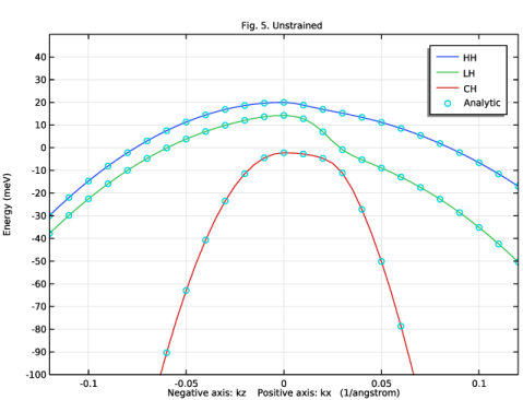
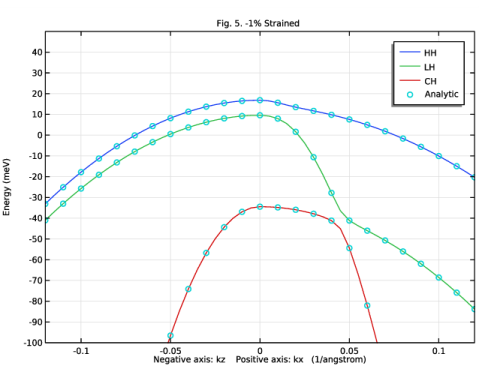
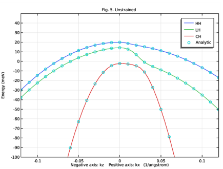
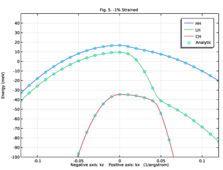
In the associated text field, type Negative axis: kz Positive axis: kx (1/angstrom).
7
Select the y-axis label check box.
8
9
Locate the Axis section. Select the Manual axis limits check box.
10
In the x minimum text field, type -0.12.
11
In the x maximum text field, type 0.12.
12
In the y minimum text field, type -100.
13
In the y maximum text field, type 50.
Global 1 - Schrödinger Eq. HH
1
Right-click Fig. 5. Unstrained and choose Global.
2
In the Settings window for Global, type Global 1 - Schrödinger Eq. HH in the Label text field.
3
Locate the Data section. From the Dataset list, choose Study 1: Fig. 5. Schrödinger Eq./Solution 1 (sol1).
4
From the Parameter selection (epsxx) list, choose First.
5
From the Eigenvalue selection list, choose Last.
6
Locate the y-Axis Data section. Click  Clear Table.
7
8
Locate the x-Axis Data section. From the Axis source data list, choose All solutions.
9
From the Parameter list, choose Expression.
10
In the Expression text field, type kp/1[angstrom^-1].
Global 1 - Schrödinger Eq. LH
1
Right-click Global 1 - Schrödinger Eq. HH and choose Duplicate.
2
In the Settings window for Global, type Global 1 - Schrödinger Eq. LH in the Label text field.
3
Locate the Data section. From the Eigenvalue selection list, choose Manual.
4
In the Eigenvalue indices (1-3) text field, type 2.
5
Locate the y-Axis Data section. In the table, enter the following settings:
Global 1 - Schrödinger Eq. CH
1
Right-click Global 1 - Schrödinger Eq. LH and choose Duplicate.
2
In the Settings window for Global, type Global 1 - Schrödinger Eq. CH in the Label text field.
3
Locate the Data section. From the Eigenvalue selection list, choose First.
4
Locate the y-Axis Data section. In the table, enter the following settings:
Duplicate the plot for the strained case. Change the plot label and the selection of the strain parameter epsxx.
Fig. 5. -1% Strained
1
In the Model Builder window, right-click Fig. 5. Unstrained and choose Duplicate.
2
In the Settings window for 1D Plot Group, type Fig. 5. -1% Strained in the Label text field.
Global 1 - Schrödinger Eq. HH
1
In the Model Builder window, expand the Fig. 5. -1% Strained node, then click Global 1 - Schrödinger Eq. HH.
2
In the Settings window for Global, locate the Data section.
3
From the Parameter selection (epsxx) list, choose Last.
Global 1 - Schrödinger Eq. LH
1
In the Model Builder window, click Global 1 - Schrödinger Eq. LH.
2
In the Settings window for Global, locate the Data section.
3
From the Parameter selection (epsxx) list, choose Last.
Global 1 - Schrödinger Eq. CH
1
In the Model Builder window, click Global 1 - Schrödinger Eq. CH.
2
In the Settings window for Global, locate the Data section.
3
From the Parameter selection (epsxx) list, choose Last.
Now set up a study to solve the analytic 3X3 matrix equation configured with the global equation. Use the All eigenvalue option to obtain all 3 eigenvalues of the 3X3 matrix equation.
Add Study
1
In the Home toolbar, click  Add Study to open the Add Study window.
2
Go to the Add Study window.
3
Find the Studies subsection. In the Select Study tree, select Empty Study.
4
Click Add Study in the window toolbar.
5
In the Home toolbar, click  Add Study to close the Add Study window.
Study 1: Fig. 5. Schrödinger Eq.
Step 1: Eigenvalue
In the Model Builder window, under Study 1: Fig. 5. Schrödinger Eq. right-click Step 1: Eigenvalue and choose Copy.
Study 2: Fig. 5. Analytic
1
In the Model Builder window, click Study 2.
2
In the Settings window for Study, type Study 2: Fig. 5. Analytic in the Label text field.
3
Locate the Study Settings section. Clear the Generate default plots check box.
4
Right-click Study 2: Fig. 5. Analytic and choose Paste Eigenvalue.
Step 1: Eigenvalue
1
In the Settings window for Eigenvalue, locate the Study Settings section.
2
From the Eigenvalue search method list, choose All (filled matrix).
3
Locate the Physics and Variables Selection section. In the table, enter the following settings:
4
Locate the Study Extensions section. In the table, enter the following settings:
5
In the Home toolbar, click  Compute.
Add the analytic solution to the 2 plots to compare with the numerical solution.
Results
Global 1 - Analytic
1
In the Model Builder window, right-click Global 1 - Schrödinger Eq. CH and choose Duplicate.
2
In the Settings window for Global, type Global 1 - Analytic in the Label text field.
3
Locate the Data section. From the Dataset list, choose Study 2: Fig. 5. Analytic/Solution 2 (sol2).
4
From the Eigenvalue selection list, choose All.
5
Locate the y-Axis Data section. In the table, enter the following settings:
6
Click to expand the Coloring and Style section. Find the Line style subsection. From the Line list, choose None.
7
Find the Line markers subsection. From the Marker list, choose Circle.
8
In the Fig. 5. Unstrained toolbar, click  Plot.
9
Right-click Global 1 - Analytic and choose Copy.
Global 1 - Analytic
1
In the Model Builder window, right-click Fig. 5. -1% Strained and choose Paste Global.
2
In the Settings window for Global, locate the Data section.
3
From the Parameter selection (epsxx) list, choose Last.
4
In the Fig. 5. -1% Strained toolbar, click  Plot.
Add a new study to compute the 2D band structure in the kx-kz plane, first using the Schrödinger equation.
Add Study
1
In the Home toolbar, click  Add Study to open the Add Study window.
2
Go to the Add Study window.
3
Find the Studies subsection. In the Select Study tree, select Empty Study.
4
Click Add Study in the window toolbar.
5
In the Home toolbar, click  Add Study to close the Add Study window.
Study 3: 2D Dispersion Schrödinger Eq.
1
In the Settings window for Study, type Study 3: 2D Dispersion Schrödinger Eq. in the Label text field.
2
Locate the Study Settings section. Clear the Generate default plots check box.
Study 1: Fig. 5. Schrödinger Eq.
Step 1: Eigenvalue
In the Model Builder window, under Study 1: Fig. 5. Schrödinger Eq. right-click Step 1: Eigenvalue and choose Copy.
Study 3: 2D Dispersion Schrödinger Eq.
In the Model Builder window, right-click Study 3: 2D Dispersion Schrödinger Eq. and choose Paste Eigenvalue.
Step 1: Eigenvalue
1
In the Settings window for Eigenvalue, locate the Study Extensions section.
2
3
In the Home toolbar, click  Compute.
Create one table for each band to plot the 2D band structure using the Table Surface plot type for the 3 hole bands. First the heavy hole band (HH).
Results
Evaluation Group 1: HH
1
In the Results toolbar, click  Evaluation Group.
2
In the Settings window for Evaluation Group, type Evaluation Group 1: HH in the Label text field.
3
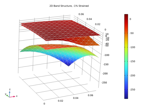
Locate the Data section. From the Dataset list, choose Study 3: 2D Dispersion Schrödinger Eq./Solution 3 (sol3).
4
From the Eigenvalue selection list, choose Last.
Global Evaluation 1: Schrödinger eq.
1
Right-click Evaluation Group 1: HH and choose Global Evaluation.
2
In the Settings window for Global Evaluation, type Global Evaluation 1: Schrödinger eq. in the Label text field.
3
Locate the Expressions section. Click  Clear Table.
4
5
In the Evaluation Group 1: HH toolbar, click  Evaluate.
Table
1
Go to the Table window.
2
Click Table Surface in the window toolbar.
Results
Table Surface 1: HH (Schr)
1
In the Model Builder window, under Results>2D Plot Group 3 click Table Surface 1.
2
In the Settings window for Table Surface, type Table Surface 1: HH (Schr) in the Label text field.
3
Locate the Data section. From the Data column list, choose HH (Schr).
Height Expression 1
Right-click Table Surface 1: HH (Schr) and choose Height Expression.
2D Band Structure, -1% Strained
1
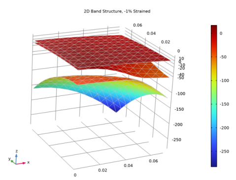
In the Settings window for 2D Plot Group, type 2D Band Structure, -1% Strained in the Label text field.
2
Click to expand the Title section. From the Title type list, choose Label.
Then the light hole band (LH).
Evaluation Group 2: LH
1
In the Model Builder window, right-click Evaluation Group 1: HH and choose Duplicate.
2
In the Settings window for Evaluation Group, type Evaluation Group 2: LH in the Label text field.
3
Locate the Data section. From the Eigenvalue selection list, choose Manual.
4
In the Eigenvalue indices (1-3) text field, type 2.
Global Evaluation 1: Schrödinger eq.
1
In the Model Builder window, expand the Evaluation Group 2: LH node, then click Global Evaluation 1: Schrödinger eq..
2
In the Settings window for Global Evaluation, locate the Expressions section.
3
4
In the Evaluation Group 2: LH toolbar, click  Evaluate.
Table Surface 2: LH (Schr)
1
In the Model Builder window, right-click Table Surface 1: HH (Schr) and choose Duplicate.
2
In the Settings window for Table Surface, type Table Surface 2: LH (Schr) in the Label text field.
3
Locate the Data section. From the Evaluation group list, choose Evaluation Group 2: LH.
4
Click to expand the Inherit Style section. From the Plot list, choose Table Surface 1: HH (Schr).
Then the crystal-field split-off hole band (CH).
Evaluation Group 3: CH
1
In the Model Builder window, right-click Evaluation Group 2: LH and choose Duplicate.
2
In the Settings window for Evaluation Group, type Evaluation Group 3: CH in the Label text field.
3
Locate the Data section. From the Eigenvalue selection list, choose First.
Global Evaluation 1: Schrödinger eq.
1
In the Model Builder window, expand the Evaluation Group 3: CH node, then click Global Evaluation 1: Schrödinger eq..
2
In the Settings window for Global Evaluation, locate the Expressions section.
3
4
In the Evaluation Group 3: CH toolbar, click  Evaluate.
Table Surface 3: CH (Schr)
1
In the Model Builder window, right-click Table Surface 2: LH (Schr) and choose Duplicate.
2
In the Settings window for Table Surface, type Table Surface 3: CH (Schr) in the Label text field.
3
Locate the Data section. From the Evaluation group list, choose Evaluation Group 3: CH.
4
In the 2D Band Structure, -1% Strained toolbar, click  Plot.
Finally set up a study to compute the 2D band structure in the kx-kz plane using the global equation of the analytic formula.
Add Study
1
In the Home toolbar, click  Add Study to open the Add Study window.
2
Go to the Add Study window.
3
Find the Studies subsection. In the Select Study tree, select Empty Study.
4
Click Add Study in the window toolbar.
5
In the Home toolbar, click  Add Study to close the Add Study window.
Study 4: 2D Dispersion Analytic
1
In the Settings window for Study, type Study 4: 2D Dispersion Analytic in the Label text field.
2
Locate the Study Settings section. Clear the Generate default plots check box.
Study 3: 2D Dispersion Schrödinger Eq.
Step 1: Eigenvalue
In the Model Builder window, under Study 3: 2D Dispersion Schrödinger Eq. right-click Step 1: Eigenvalue and choose Copy.
Study 4: 2D Dispersion Analytic
In the Model Builder window, right-click Study 4: 2D Dispersion Analytic and choose Paste Eigenvalue.
Step 1: Eigenvalue
1
In the Settings window for Eigenvalue, locate the Study Settings section.
2
From the Eigenvalue search method list, choose All (filled matrix).
3
Locate the Physics and Variables Selection section. In the table, enter the following settings:
4
In the Home toolbar, click  Compute.
Similarly create one table for each band to plot the analytic 2D band structure using the Table Surface plot type for the 3 hole bands. Use the Wireframe option for the analytic result to compare to the numerical result by overlaying the plotted surfaces. First the heavy hole band (HH).
Results
Global Evaluation 2: Analytic
1
In the Model Builder window, right-click Global Evaluation 1: Schrödinger eq. and choose Duplicate.
2
In the Settings window for Global Evaluation, type Global Evaluation 2: Analytic in the Label text field.
3
Locate the Data section. From the Dataset list, choose Study 4: 2D Dispersion Analytic/Solution 4 (sol4).
4
From the Eigenvalue selection list, choose Last.
5
Locate the Expressions section. In the table, enter the following settings:
6
In the Evaluation Group 1: HH toolbar, click  Evaluate.
Table Surface 4: HH (Anal)
1
In the Model Builder window, right-click Table Surface 1: HH (Schr) and choose Duplicate.
2
In the Settings window for Table Surface, type Table Surface 4: HH (Anal) in the Label text field.
3
Locate the Data section. From the Data column list, choose HH (Anal).
4
Locate the Coloring and Style section. From the Coloring list, choose Uniform.
5
From the Color list, choose Gray.
6
Select the Wireframe check box.
7
Locate the Inherit Style section. From the Plot list, choose Table Surface 1: HH (Schr).
8
Clear the Color check box.
Then the light hole band (LH).
Global Evaluation 2: Analytic
1
In the Model Builder window, right-click Global Evaluation 1: Schrödinger eq. and choose Duplicate.
2
In the Settings window for Global Evaluation, type Global Evaluation 2: Analytic in the Label text field.
3
Locate the Data section. From the Dataset list, choose Study 4: 2D Dispersion Analytic/Solution 4 (sol4).
4
From the Eigenvalue selection list, choose Manual.
5
In the Eigenvalue indices (1-3) text field, type 2.
6
Locate the Expressions section. In the table, enter the following settings:
7
In the Evaluation Group 2: LH toolbar, click  Evaluate.
Table Surface 5: LH (Anal)
1
In the Model Builder window, right-click Table Surface 4: HH (Anal) and choose Duplicate.
2
In the Settings window for Table Surface, type Table Surface 5: LH (Anal) in the Label text field.
3
Locate the Data section. From the Evaluation group list, choose Evaluation Group 2: LH.
Then the crystal-field split-off hole band (CH).
Global Evaluation 2: Analytic
1
In the Model Builder window, right-click Global Evaluation 1: Schrödinger eq. and choose Duplicate.
2
In the Settings window for Global Evaluation, type Global Evaluation 2: Analytic in the Label text field.
3
Locate the Data section. From the Dataset list, choose Study 4: 2D Dispersion Analytic/Solution 4 (sol4).
4
From the Eigenvalue selection list, choose First.
5
Locate the Expressions section. In the table, enter the following settings:
6
In the Evaluation Group 3: CH toolbar, click  Evaluate.
Table Surface 6: CH (Anal)
1
In the Model Builder window, right-click Table Surface 5: LH (Anal) and choose Duplicate.
2
In the Settings window for Table Surface, type Table Surface 6: CH (Anal) in the Label text field.
3
Locate the Data section. From the Evaluation group list, choose Evaluation Group 3: CH.
4
In the 2D Band Structure, -1% Strained toolbar, click  Plot.
Use mouse drag to rotate the energy surfaces around to take a look. Ignore the following instructions on setting camera views.
5
In the Model Builder window, expand the Results>Views node.
Camera
1
In the Model Builder window, expand the Results>Views>View 3D 3 node, then click Camera.
2
In the Settings window for Camera, locate the Position section.
3
In the x text field, type -0.2.
4
In the y text field, type -0.4.
5
In the z text field, type 0.2.
6
Locate the Up Vector section. In the x text field, type 0.1.
7
In the y text field, type 0.3.
8
In the z text field, type 0.95.
9
Click  Update.