PDF

Response of a Rotor Under the Influence of Seal Forces
Introduction
In fluid seals found in axial compressors, two types of fluid forces can be distinguished. The first type of force directly opposes the lateral motion of the rotor, and it is modeled using equivalent direct stiffness and damping coefficients. The second force type acts in the circumferential direction of the rotor. This force is modeled with cross stiffness and damping coefficients. The first type of force always tends to stabilize the rotor, whereas the second type may have destabilizing effects under certain conditions.
In this example, an axial compressor is modeled using the Beam Rotor interface. The compressor has ten impeller stages with a seal located near each impeller. The compressor model also includes a balance piston seal located at the end of all impeller stages. The time-dependent response of the compressor is studied for a gradually increasing rotor speed. In order to compare the effect of the seals on the rotor response two studies are performed, one without and one with the seals included. In this case, the seals have a stabilizing effect on the compressor as the displacement amplitude is significantly smaller in the presence of the seals.
Model Definition
The model consists of an axial compressor with ten impeller stages. The overall configuration is shown in Figure 1. The rotor is supported with two hydrodynamic bearings. Each impeller stage is accompanied by a seal to avoid flow leakage. In addition, there is a balance piston seal at the end of the impeller stages. The rotor’s weight is supported by the bearings and the seals. The impellers are modeled with small mass eccentricities.
Figure 1: Rotor geometry.
Shaft Properties
The diameter of the rotor shaft varies along its length. Thus, to more easily apply different properties, the rotor axis is divided into multiple segments separated by various support points. Some of these points separate segments with different shaft diameters, and others mark the locations of seals, impellers and bearings. The coordinates of the various stations are given in Table 1.
The shaft diameters for the different segments are given in the Table 2.
Impeller Properties
The properties of the impellers are given in the Table 3.
All impellers are located between stations 5 and 6, and they are equidistantly spaced in this shaft segment. The first impeller is located at a distance of 62 mm from station 5. The axial length of each impeller is 80 mm.
Bearing Properties
The rotor is supported on two plain hydrodynamic journal bearings. The first bearing is located in the middle of stations 3 and 4. The second bearing is located adjacent to station 8 such that the right end of the bearing touches this station. The length of each bearings is 96 mm. The radius of both bearings is 52.5 mm and the radial clearance in each bearing is 0.15 mm. The viscosity of the bearing lubricant is 0.0414 Pa·s.
Seal Properties
The properties of the seals are given in the Table 4.
The annular seals are equidistantly spaced between stations 5 and 6 on the rotor with the left end of the first seal starting at station 5. The right end of the balance piston seal is located at station 7. The density and viscosity of the seal fluid are 800 kg/m3 and 0.02 Pa·s, respectively.
Results and Discussion
Figure 2 shows the von Mises stress in the rotor after including the seal forces at t=2 seconds. The response appears to be similar to the first bending mode of the rotor. The rotor geometry is also shown below the stress plot.
Figure 2: von Mises stress in the rotor with seals at t=2 secconds.
The orbit of the rotor near the left bearing is shown in Figure 3. In the presence of seals, the displacement amplitude of the whirl is considerably smaller. The orbit plot indicates a growing whirl amplitude in the absence of seals towards the end of the simulation.
Figure 3: Orbit of the rotor in the bearing with and without seals.
The stiffness and damping coefficients of seals play an important role in dictating the rotor stability. The direct and cross stiffnesses for the balance piston seal are shown in Figure 4. Clearly, the direct rotor stiffness decreases with rotor speed whereas the cross stiffness increases. Also, the change in the cross stiffness is more sensitive to the change in speed as compared to the direct stiffness.
Figure 4: Stiffness of the balance piston seal.
The vertical displacement at impeller 5 is compared with and without seals in Figure 5. From this plot also we can deduce that the vibration amplitudes of the rotor are significantly larger without seals. At higher rotor speeds, the amplitude of the displacement is growing without seals.
Figure 5: Comparison of the vertical displacement of the rotor at impeller 5.
Application Library path: Rotordynamics_Module/Tutorials/rotor_stability_with_seal
Modeling Instructions
From the File menu, choose New.
New
In the New window, click  Model Wizard.
Model Wizard
1
In the Model Wizard window, click  3D.
2
In the Select Physics tree, select Structural Mechanics>Rotordynamics>Beam Rotor (rotbm).
3
Click Add.
4
Click  Study.
5
In the Select Study tree, select General Studies>Time Dependent.
6
Global Definitions
Parameters: Stations
Start by importing the parameters for the rotor, bearings, seals and impellers.
1
In the Model Builder window, under Global Definitions click Parameters 1.
2
In the Settings window for Parameters, locate the Parameters section.
3
Click  Load from File.
4
5
In the Label text field, type Parameters: Stations.
Parameters: Rotor Diameters
1
In the Home toolbar, click  Parameters and choose Add>Parameters.
2
In the Settings window for Parameters, locate the Parameters section.
3
Click  Load from File.
4
5
In the Label text field, type Parameters: Rotor Diameters.
Parameters: Bearings
1
In the Home toolbar, click  Parameters and choose Add>Parameters.
2
In the Settings window for Parameters, locate the Parameters section.
3
Click  Load from File.
4
5
In the Label text field, type Parameters: Bearings.
Parameters: Impellers
1
In the Home toolbar, click  Parameters and choose Add>Parameters.
2
In the Settings window for Parameters, locate the Parameters section.
3
Click  Load from File.
4
5
In the Label text field, type Parameters: Impellers.
Parameters: Seals
1
In the Home toolbar, click  Parameters and choose Add>Parameters.
2
In the Settings window for Parameters, locate the Parameters section.
3
Click  Load from File.
4
5
In the Label text field, type Parameters: Seals.
Geometry 1
Polygon 1 (pol1)
1
In the Geometry toolbar, click  More Primitives and choose Polygon.
2
In the Settings window for Polygon, locate the Coordinates section.
3
From the Data source list, choose Vectors.
Use the station coordinates together with location of bearings, seals and impellers to create a 1D representation of the rotor.
4
In the x text field, type x1 x2 x3 xb1 x4 x5 xs1 xd1 xs2 xd2 xs3 xd3 xs4 xd4 xs5 xd5 xs6 xd6 xs7 xd7 xs8 xd8 xs9 xd9 xs10 xd10 x6 xp x7 xb2 x8 x9 x10.
5
In the y text field, type 0.
6
In the z text field, type 0.
7
Click  Build All Objects.
Definitions
You can specify the diameter of the rotor between different stations by using as many Rotor Cross Section nodes as rotor segments. You can avoid many such nodes by using the interpolation function for the axial variation of the rotor diameter. You can use a small axial tolerance in the interpolation data to create the steps in the diameter near the stations.
Interpolation: Diameters
1
In the Model Builder window, expand the Component 1 (comp1)>Definitions node.
2
Right-click Definitions and choose Functions>Interpolation.
Import the text file containing the axial variation of the diameter.
3
In the Settings window for Interpolation, locate the Definition section.
4
Click  Load from File.
5
6
In the Label text field, type Interpolation: Diameters.
7
Locate the Definition section. In the Function name text field, type dia.
8
Locate the Units section. In the Function table, enter the following settings:
9
In the Argument table, enter the following settings:
10
Materials
In the Home toolbar, click  Windows and choose Add Material from Library.
Add Material
1
Go to the Add Material window.
2
In the tree, select Built-in>Structural steel.
3
Click Add to Component in the window toolbar.
4
In the Home toolbar, click  Add Material to close the Add Material window.
Beam Rotor (rotbm)
The rotor speed is linearly increased from 1000 rpm to 10000 rpm in 2 seconds.
1
In the Model Builder window, under Component 1 (comp1) click Beam Rotor (rotbm).
2
In the Settings window for Beam Rotor, locate the Rotor Speed section.
3
In the text field, type 4500[rpm/s]*t+1000[rpm].
Rotor Cross Section 1
Use the interpolation function with the axial coordinate as argument to specify the axial variation of the diameter.
1
In the Model Builder window, under Component 1 (comp1)>Beam Rotor (rotbm) click Rotor Cross Section 1.
2
In the Settings window for Rotor Cross Section, locate the Cross-Section Definition section.
3
In the do text field, type dia(x).
Gravity 1
1
In the Physics toolbar, click  Edges and choose Gravity.
2
In the Settings window for Gravity, locate the Edge Selection section.
3
From the Selection list, choose All edges.
Journal Bearing 1
1
In the Physics toolbar, click  Points and choose Journal Bearing.
2
3
In the Settings window for Journal Bearing, locate the Bearing Properties section.
4
From the Bearing model list, choose Plain hydrodynamic.
5
From the μ list, choose User defined. In the associated text field, type mu_b.
6
In the C text field, type Cb.
7
In the R text field, type Rb.
8
In the L text field, type Lb.
9
Clear the Include bending stiffness check box.
You use disk features to specify the impeller properties.
Disk 1
1
In the Physics toolbar, click  Points and choose Disk.
2
3
In the Settings window for Disk, locate the Disk Properties section.
4
In the m text field, type md1.
5
In the Ip text field, type 2*Jd1.
6
In the Id text field, type Jd1.
7
From the Center of mass list, choose Offset from selected points.
8
In the zr text field, type e1.
Disk 2-9
1
Right-click Disk 1 and choose Duplicate.
2
In the Settings window for Disk, type Disk 2-9 in the Label text field.
3
Locate the Point Selection section. Click  Clear Selection.
4
5
Locate the Disk Properties section. In the m text field, type md2.
6
In the Ip text field, type 2*Jd2.
7
In the Id text field, type Jd2.
Disk 10
1
In the Model Builder window, under Component 1 (comp1)>Beam Rotor (rotbm) right-click Disk 1 and choose Duplicate.
2
In the Settings window for Disk, type Disk 10 in the Label text field.
3
Locate the Point Selection section. Click  Clear Selection.
4
5
Locate the Disk Properties section. In the m text field, type md10.
6
In the Ip text field, type 2*Jd10.
7
In the Id text field, type Jd10.
Disk 1, Disk 10, Disk 2-9
1
In the Model Builder window, under Component 1 (comp1)>Beam Rotor (rotbm), Ctrl-click to select Disk 1, Disk 2-9, and Disk 10.
2
Impellers
In the Settings window for Group, type Impellers in the Label text field.
Study 1
Step 1: Time Dependent
1
In the Model Builder window, under Study 1 click Step 1: Time Dependent.
2
In the Settings window for Time Dependent, locate the Study Settings section.
3
In the Output times text field, type range(0,5e-4,2).
Solution 1 (sol1)
1
In the Study toolbar, click  Show Default Solver.
2
In the Model Builder window, expand the Solution 1 (sol1) node.
3
In the Model Builder window, expand the Study 1>Solver Configurations>Solution 1 (sol1)>Time-Dependent Solver 1 node, then click Fully Coupled 1.
4
In the Settings window for Fully Coupled, click to expand the Method and Termination section.
Use the Automatic Newton solver to capture the nonlinearities in the bearings.
5
From the Nonlinear method list, choose Automatic (Newton).
6
In the Model Builder window, click Study 1.
7
In the Settings window for Study, type Study: without Seal in the Label text field.
8
In the Study toolbar, click  Compute.
Follow the instructions to create the orbit plot at the bearing location.
Results
Orbit
1
In the Home toolbar, click  Add Plot Group and choose 1D Plot Group.
2
In the Settings window for 1D Plot Group, type Orbit in the Label text field.
Point Graph 1
1
Right-click Orbit and choose Point Graph.
2
3
In the Settings window for Point Graph, locate the y-Axis Data section.
4
In the Expression text field, type w/Cb.
5
Locate the x-Axis Data section. From the Parameter list, choose Expression.
6
In the Expression text field, type v/Cb.
7
Click to expand the Coloring and Style section. In the Width text field, type 3.
8
Click to expand the Legends section. Select the Show legends check box.
9
From the Legends list, choose Manual.
10
Orbit
1
In the Model Builder window, click Orbit.
2
In the Settings window for 1D Plot Group, locate the Axis section.
3
Select the Preserve aspect ratio check box.
4
In the Orbit toolbar, click  Plot.
The study without seals is complete now. Next, add seals in the model and perform a new study to analyze their influence.
Beam Rotor (rotbm)
Liquid Annular Seal 1
1
In the Physics toolbar, click  Points and choose Liquid Annular Seal.
2
In the Settings window for Liquid Annular Seal, locate the Geometric Properties section.
3
In the R text field, type ds/2.
4
In the Ls text field, type Ls.
5
In the C text field, type Cs.
6
Locate the Fluid Properties section. From the ρ list, choose User defined. In the associated text field, type rho_f.
7
From the μ list, choose User defined. In the associated text field, type mu_f.
8
Locate the Flow Properties section. In the ΔP text field, type dPs.
9
In the V0 text field, type 60.
The seals near the impellers are short in length. Use the Childs’ model to account for the inlet swirling effect in these seals.
10
Locate the Seal Model section. From the list, choose Childs.
11
Locate the Flow Properties section. In the α text field, type 0.7.
12
The seals at each stage are identical. Create 10 such features by duplicating and changing the selection.
Liquid Annular Seal 2
1
Right-click Liquid Annular Seal 1 and choose Duplicate.
2
In the Settings window for Liquid Annular Seal, locate the Point Selection section.
3
Click  Clear Selection.
4
Liquid Annular Seal 3
1
Right-click Liquid Annular Seal 2 and choose Duplicate.
2
Liquid Annular Seal 4
1
Right-click Liquid Annular Seal 3 and choose Duplicate.
2
In the Settings window for Liquid Annular Seal, locate the Point Selection section.
3
Click  Clear Selection.
4
Liquid Annular Seal 1, Liquid Annular Seal 2, Liquid Annular Seal 3, Liquid Annular Seal 4
1
In the Model Builder window, under Component 1 (comp1)>Beam Rotor (rotbm), Ctrl-click to select Liquid Annular Seal 1, Liquid Annular Seal 2, Liquid Annular Seal 3, and Liquid Annular Seal 4.
2
Liquid Annular Seal 5
1
In the Settings window for Liquid Annular Seal, locate the Point Selection section.
2
Click  Clear Selection.
3
Liquid Annular Seal 6
1
In the Model Builder window, click Liquid Annular Seal 6.
2
In the Settings window for Liquid Annular Seal, locate the Point Selection section.
3
Click  Clear Selection.
4
Liquid Annular Seal 7
1
In the Model Builder window, click Liquid Annular Seal 7.
2
In the Settings window for Liquid Annular Seal, locate the Point Selection section.
3
Click  Clear Selection.
4
Liquid Annular Seal 8
1
In the Model Builder window, click Liquid Annular Seal 8.
2
In the Settings window for Liquid Annular Seal, locate the Point Selection section.
3
Click  Clear Selection.
4
Liquid Annular Seal 9
1
Right-click Component 1 (comp1)>Beam Rotor (rotbm)>Liquid Annular Seal 8 and choose Duplicate.
2
In the Settings window for Liquid Annular Seal, locate the Point Selection section.
3
Click  Clear Selection.
4
Liquid Annular Seal 10
1
Right-click Liquid Annular Seal 9 and choose Duplicate.
2
In the Settings window for Liquid Annular Seal, locate the Point Selection section.
3
Click  Clear Selection.
4
Liquid Annular Seal 1, Liquid Annular Seal 10, Liquid Annular Seal 2, Liquid Annular Seal 3, Liquid Annular Seal 4, Liquid Annular Seal 5, Liquid Annular Seal 6, Liquid Annular Seal 7, Liquid Annular Seal 8, Liquid Annular Seal 9
1
In the Model Builder window, under Component 1 (comp1)>Beam Rotor (rotbm), Ctrl-click to select Liquid Annular Seal 1, Liquid Annular Seal 2, Liquid Annular Seal 3, Liquid Annular Seal 4, Liquid Annular Seal 5, Liquid Annular Seal 6, Liquid Annular Seal 7, Liquid Annular Seal 8, Liquid Annular Seal 9, and Liquid Annular Seal 10.
2
Seals
1
In the Settings window for Group, type Seals in the Label text field.
2
In the Model Builder window, collapse the Seals node.
Next, add a balance piston seal.
Balance Piston Seal
1
In the Physics toolbar, click  Points and choose Liquid Annular Seal.
2
In the Settings window for Liquid Annular Seal, locate the Geometric Properties section.
3
In the R text field, type dp/2.
4
In the Ls text field, type Lp.
5
In the C text field, type Cp.
6
Locate the Fluid Properties section. From the ρ list, choose User defined. In the associated text field, type rho_f.
7
From the μ list, choose User defined. In the associated text field, type mu_f.
8
Locate the Flow Properties section. In the ΔP text field, type dPp.
9
In the V0 text field, type 90.
10
11
In the Label text field, type Balance Piston Seal.
The balance piston seal has a finite length. The Black and Jenssen model is preferred in this case.
Root
In the Home toolbar, click  Windows and choose Add Study.
Add Study
1
Go to the Add Study window.
2
Find the Studies subsection. In the Select Study tree, select General Studies>Time Dependent.
3
Click Add Study in the window toolbar.
4
In the Home toolbar, click  Add Study to close the Add Study window.
Study 2
Step 1: Time Dependent
1
In the Settings window for Time Dependent, locate the Study Settings section.
2
In the Output times text field, type range(0,5e-4,2).
Solution 2 (sol2)
1
In the Study toolbar, click  Show Default Solver.
2
In the Model Builder window, expand the Solution 2 (sol2) node.
3
In the Model Builder window, expand the Study 2>Solver Configurations>Solution 2 (sol2)>Time-Dependent Solver 1 node, then click Fully Coupled 1.
4
In the Settings window for Fully Coupled, locate the Method and Termination section.
5
From the Nonlinear method list, choose Automatic (Newton).
6
In the Model Builder window, click Study 2.
7
In the Settings window for Study, type Study: with Seal in the Label text field.
8
In the Study toolbar, click  Compute.
Results
Stress (rotbm) 1
The stress in the rotor is a default plot, see Figure 2.
1
Click the  Zoom Extents button in the Graphics toolbar.
Point Graph 1
Duplicate the Point Graph 1 in the Orbit plot and change the solution to compare the response with and without seals. This plot is shown in Figure 3.
Point Graph 2
1
In the Model Builder window, under Results>Orbit right-click Point Graph 1 and choose Duplicate.
2
In the Settings window for Point Graph, locate the Data section.
3
From the Dataset list, choose Study: with Seal/Solution 2 (sol2).
4
Locate the Legends section. In the table, enter the following settings:
5
In the Orbit toolbar, click  Plot.
The seal stiffness plays an important role in determining the response of the rotor. Use the following instructions to plot the variation of the balance piston seal stiffness with rotor speed as shown in Figure 4.
Balance Piston Seal Stiffness
1
In the Home toolbar, click  Add Plot Group and choose 1D Plot Group.
2
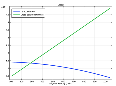
In the Settings window for 1D Plot Group, type Balance Piston Seal Stiffness in the Label text field.
3
Locate the Data section. From the Dataset list, choose Study: with Seal/Solution 2 (sol2).
Global 1
1
Right-click Balance Piston Seal Stiffness and choose Global.
2
In the Settings window for Global, click Replace Expression in the upper-right corner of the y-Axis Data section. From the menu, choose Component 1 (comp1)>Beam Rotor>Balance Piston Seal>rotbm.las11.Kd - Direct stiffness - N/m.
3
Click Add Expression in the upper-right corner of the y-Axis Data section. From the menu, choose Component 1 (comp1)>Beam Rotor>Balance Piston Seal>rotbm.las11.kc - Cross-coupled stiffness - N/m.
4
Locate the x-Axis Data section. From the Parameter list, choose Expression.
5
In the Expression text field, type rotbm.las11.Omega.
6
Click to expand the Coloring and Style section. In the Width text field, type 3.
7
In the Balance Piston Seal Stiffness toolbar, click  Plot.
Balance Piston Seal Stiffness
1
In the Model Builder window, click Balance Piston Seal Stiffness.
2
In the Settings window for 1D Plot Group, locate the Legend section.
3
From the Position list, choose Upper left.
Use the following instructions to compare the vertical displacement of the rotor at impeller 5 as shown in Figure 5.
Vertical Displacement at Impeller 5
1
In the Home toolbar, click  Add Plot Group and choose 1D Plot Group.
2
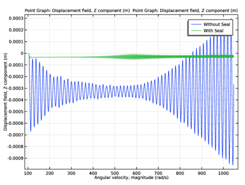
In the Settings window for 1D Plot Group, type Vertical Displacement at Impeller 5 in the Label text field.
Point Graph: Without Seal
1
Right-click Vertical Displacement at Impeller 5 and choose Point Graph.
2
In the Settings window for Point Graph, type Point Graph: Without Seal in the Label text field.
3
4
Locate the y-Axis Data section. In the Expression text field, type w.
5
Locate the x-Axis Data section. From the Parameter list, choose Expression.
6
In the Expression text field, type rotbm.Ov.
7
Locate the Legends section. Select the Show legends check box.
8
From the Legends list, choose Manual.
9
Point Graph: With Seal
1
Right-click Point Graph: Without Seal and choose Duplicate.
2
In the Settings window for Point Graph, type Point Graph: With Seal in the Label text field.
3
Locate the Data section. From the Dataset list, choose Study: with Seal/Solution 2 (sol2).
4
Locate the Legends section. In the table, enter the following settings:
5
In the Vertical Displacement at Impeller 5 toolbar, click  Plot.
Now, you can disable seals from the first study to allow the recomputation without seals.
Study: without Seal
Step 1: Time Dependent
1
In the Model Builder window, under Study: without Seal click Step 1: Time Dependent.
2
In the Settings window for Time Dependent, locate the Physics and Variables Selection section.
3
Select the Modify model configuration for study step check box.
4
In the tree, select Component 1 (Comp1)>Beam Rotor (Rotbm)>Seals and Component 1 (Comp1)>Beam Rotor (Rotbm)>Balance Piston Seal.
5
Click  Disable.