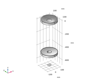
PDF

Gregory-Maksutov Telescope
Introduction
The Gregory-Maksutov telescope is a simple catadioptric telescope comprising a spherical corrector lens and a spherical primary mirror. In this example, the corrector lens and mirror are formed using the ‘Spherical Lens 3D’ and ‘Spherical Mirror 3D’ parts, respectively, from the Ray Optics Module Part Library. A cross-section of the optical design is shown in Figure 1.
Figure 1: Overview of the Gregory-Maksutov telescope.
 
The origin of the Gregory-Maksutov telescope was a desire to avoid the aspheric corrector used in the Schmidt family of telescopes. An example of this type of telescope, the Schmidt-Cassegrain Telescope, can also be found in the Ray Optics Module Application Library. At least four optical designers, including Dmitri Maksutov, found a solution involving a meniscus corrector lens in the early 1940s, and it was John Gregory who, in 1957, popularized the design used in this tutorial.
Model Definition
Details of the Gregory-Maksutov telescope used in this tutorial can be found in Ref. 1. This telescope has a 200 mm entrance aperture and an f/15 focal ratio. The detailed optical prescription is given in Table 1.
75.0000
20.0000
70.0000
268.6151
30.0000
200.1688
286.1193
453.0476
208.0594
Primary mirror1
1111.6100
453.0476
217.0732
Secondary mirror2
286.1193
453.0476
48.2704
200.0000
26.0556

1
The primary mirror central hole diameter is d = 60.0 mm.

2
The secondary mirror surface is on surface 2 of the corrector.

The telescope geometry is constructed using parts from the Ray Optics Module Part Library. The meniscus corrector is created using an instance of the Spherical Lens 3D part, whereas the Spherical Mirror 3D part is used to create the primary mirror. The secondary mirror is defined by an aperture on surface 2 of the meniscus corrector. That is, the surface is intended to be reflective within this aperture. Other predefined selections on this part are used to define the corrector clear apertures as well as the central obstruction.
When constructing a geometry in COMSOL to be used in a Geometrical Optics ray trace, it is important to appreciate that the order in which optical elements are placed in a geometry sequence does not affect the results of the trace. However, it is convenient to place optical elements relative to one another. This can be achieved by taking one of the built-in work planes in a Part Instance as the reference for the placement of the next Part Instance. The resulting Gregory-Maksutov telescope geometry sequence is shown in Figure 2. Detailed instructions for creating the geometry can be found in Appendix — Geometry Instructions.
Figure 2: The Gregory-Maksutov telescope geometry sequence.
Figure 3: The mesh for the Gregory-Maksutov telescope. Note that the default Physics-based mesh should be slightly refined in order to improve the ray tracing accuracy.
Results and Discussion
A ray trace has been performed using three wavelengths (486 nm, 546 nm, and 656 nm) at three field angles (0, 0.125, and 0.25 degrees). Figure 4 shows the resulting ray trajectories; the Color Expression represents the ray positions on the image surface.
In Figure 5, the intersection of the rays with the image surface is shown. This spot diagram shows each of the three field angles, where the Color Expression is the wavelength.
 
Figure 4: Ray diagram for the Gregory-Maksutov telescope colored by radial distance from the centroid.
Figure 5: Spot diagram for the Gregory-Maksutov telescope colored by wavelength. For reference, the Airy disc is shown in the lower-left corner.
 
Reference
1. G.H. Smith, R. Ceragioli, and R. Berry, Telescopes, Eyepieces, and Astrographs: Design, Analysis, and Performance of Modern Astronomical Optics, Willmann-Bell, 2012.
Application Library path: Ray_Optics_Module/Lenses_Cameras_and_Telescopes/gregory_maksutov_telescope
Modeling Instructions
From the File menu, choose New.
New
In the New window, click  Model Wizard.
Model Wizard
1
In the Model Wizard window, click  3D.
2
In the Select Physics tree, select Optics>Ray Optics>Geometrical Optics (gop).
3
Click Add.
4
Click  Study.
5
In the Select Study tree, select Preset Studies for Selected Physics Interfaces>Ray Tracing.
6
Global Definitions
Parameters 1: Lens Prescription
1
In the Model Builder window, under Global Definitions click Parameters 1.
2
In the Settings window for Parameters, type Parameters 1: Lens Prescription in the Label text field. The lens prescription will be added when the geometry sequence is inserted in the following section.
Parameters 2: General
The simulation parameters can be loaded from a text file.
1
In the Home toolbar, click  Parameters and choose Add>Parameters.
2
In the Settings window for Parameters, type Parameters 2: General in the Label text field.
3
Locate the Parameters section. Click  Load from File.
4
Component 1 (comp1)
1
In the Model Builder window, click Component 1 (comp1).
2
In the Settings window for Component, locate the Curved Mesh Elements section.
3
From the Geometry shape function list, choose Cubic Lagrange. The ray tracing algorithm used by the Geometrical Optics interface computes the refracted ray direction based on a discretized geometry via the underlying finite element mesh. A cubic geometry shape order usually introduces less discretization error compared to the default, which uses linear and quadratic polynomials.
Gregory-Maksutov Telescope
Insert the prepared geometry sequence from file. You can read the instructions for creating the geometry in the appendix. Following insertion, the lens definitions will be available in the Parameters node.
1
In the Model Builder window, under Component 1 (comp1) click Geometry 1.
2
In the Settings window for Geometry, locate the Units section.
3
From the Length unit list, choose mm.
4
In the Label text field, type Gregory-Maksutov Telescope.
5
In the Geometry toolbar, click Insert Sequence and choose Insert Sequence.
6
7
In the Geometry toolbar, click  Build All.
8
Click the  Orthographic Projection button in the Graphics toolbar. Compare the resulting geometry to Figure 2.
Add Material
1
In the Home toolbar, click  Add Material to open the Add Material window.
2
Go to the Add Material window.
3
In the tree, select Optical>Schott Glass>Schott N-BK7 Glass.
4
Click Add to Component in the window toolbar.
5
In the Home toolbar, click  Add Material to close the Add Material window.
Materials
Schott N-BK7 Glass (mat1)
1
In the Settings window for Material, locate the Geometric Entity Selection section.
2
From the Selection list, choose All (Corrector).
Geometrical Optics (gop)
1
In the Model Builder window, under Component 1 (comp1) click Geometrical Optics (gop).
2
3
In the Settings window for Geometrical Optics, locate the Ray Release and Propagation section.
4
From the Wavelength distribution of released rays list, choose Polychromatic, specify vacuum wavelength.
5
In the Maximum number of secondary rays text field, type 0. In this simulation stray light is not being traced, so reflected rays will not be produced at the lens surfaces.
6
Select the Use geometry normals for ray-boundary interactions check box. In this simulation, the geometry normals are used to apply the boundary conditions on all refracting surfaces. This is appropriate for the highest accuracy ray traces in single-physics simulations, where the geometry is not deformed.
Medium Properties 1
1
In the Model Builder window, under Component 1 (comp1)>Geometrical Optics (gop) click Medium Properties 1.
2
In the Settings window for Medium Properties, locate the Medium Properties section.
3
From the Refractive index of domains list, choose Get dispersion model from material. The material added above contains the optical dispersion coefficients which can be used to compute the refractive index as a function of wavelength.
Material Discontinuity 1
1
In the Model Builder window, click Material Discontinuity 1.
2
In the Settings window for Material Discontinuity, locate the Rays to Release section.
3
From the Release reflected rays list, choose Never.
Mirrors
1
In the Physics toolbar, click  Boundaries and choose Mirror.
2
In the Settings window for Mirror, type Mirrors in the Label text field.
3
Locate the Boundary Selection section. From the Selection list, choose Mirrors.
Obstructions
1
In the Physics toolbar, click  Boundaries and choose Wall.
2
In the Settings window for Wall, type Obstructions in the Label text field.
3
Locate the Boundary Selection section. From the Selection list, choose Obstructions.
4
Locate the Wall Condition section. From the Wall condition list, choose Disappear.
Image
1
In the Physics toolbar, click  Boundaries and choose Wall.
2
In the Settings window for Wall, type Image in the Label text field.
3
Locate the Boundary Selection section. From the Selection list, choose All (Image plane).
Release from Grid 1
Release rays from a set of hexapolar grids using quantities defined in the Parameters 2: General node.
1
In the Physics toolbar, click  Global and choose Release from Grid.
2
In the Settings window for Release from Grid, locate the Initial Coordinates section.
3
From the Grid type list, choose Hexapolar.
4
Specify the qc vector as
5
Specify the rc vector as
6
In the Rc text field, type P_nom/2.
7
In the Nc text field, type N_ring.
8
Locate the Ray Direction Vector section. Specify the L0 vector as
9
Locate the Vacuum Wavelength section. From the Distribution function list, choose List of values.
10
In the Values text field, type lam1 lam2 lam3. These wavelengths were defined in the Parameters 2: General node.
Release from Grid 2
1
Right-click Release from Grid 1 and choose Duplicate.
2
In the Settings window for Release from Grid, locate the Initial Coordinates section.
3
Specify the qc vector as
4
Locate the Ray Direction Vector section. Specify the L0 vector as
Release from Grid 3
1
Right-click Release from Grid 2 and choose Duplicate.
2
In the Settings window for Release from Grid, locate the Initial Coordinates section.
3
Specify the qc vector as
4
Locate the Ray Direction Vector section. Specify the L0 vector as
Mesh 1
Next, build the mesh. First, slightly refine the mesh to improve the ray tracing accuracy.
1
In the Model Builder window, under Component 1 (comp1) click Mesh 1.
2
In the Settings window for Mesh, locate the Physics-Controlled Mesh section.
3
From the Element size list, choose Finer.
4
Click  Build All. The mesh should looks like Figure 3.
Study 1
Step 1: Ray Tracing
1
In the Model Builder window, under Study 1 click Step 1: Ray Tracing.
2
In the Settings window for Ray Tracing, locate the Study Settings section.
3
From the Time-step specification list, choose Specify maximum path length.
4
From the Length unit list, choose mm.
5
In the Lengths text field, type 0 1750.
6
In the Home toolbar, click  Compute.
Results
Ray Diagram
Now, make some modifications to the default Ray Trajectories plot.
1
In the Settings window for 3D Plot Group, type Ray Diagram in the Label text field.
2
Locate the Color Legend section. Select the Show units check box.
Ray Trajectories 1
In the Model Builder window, expand the Ray Diagram node.
Color Expression 1
1
In the Model Builder window, expand the Ray Trajectories 1 node, then click Color Expression 1.
2
In the Settings window for Color Expression, locate the Expression section.
3
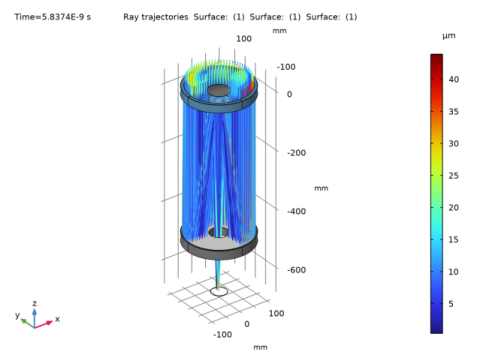
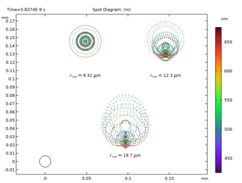
In the Expression text field, type at('last',gop.rrel). This expression gives the radial distance from the centroid of the spot on the image plane generated by each release feature.
4
From the Unit list, choose µm.
Filter 1
1
In the Model Builder window, click Filter 1.
2
In the Settings window for Filter, locate the Ray Selection section.
3
From the Rays to include list, choose Logical expression.
4
In the Logical expression for inclusion text field, type at(0,atan2(qy,qx)>-pi/2). This filter removes 1/4 of the rays so that the optical geometry is visible.
Ray Diagram
In the following we add and color surface plots to show the various telescope optical elements.
Surface 1
1
In the Model Builder window, right-click Ray Diagram and choose Surface.
2
In the Settings window for Surface, locate the Coloring and Style section.
3
From the Coloring list, choose Uniform.
4
From the Color list, choose Custom.
5
6
Click Define custom colors.
7
8
Click Add to custom colors.
9
Click Show color palette only or OK on the cross-platform desktop.
Selection 1
1
Right-click Surface 1 and choose Selection.
2
In the Settings window for Selection, locate the Selection section.
3
From the Selection list, choose Exterior (Corrector).
4
Transparency 1
In the Model Builder window, right-click Surface 1 and choose Transparency.
Surface 2
1
In the Model Builder window, right-click Ray Diagram and choose Surface.
2
In the Settings window for Surface, locate the Coloring and Style section.
3
From the Coloring list, choose Uniform.
4
From the Color list, choose Gray.
Selection 1
1
Right-click Surface 2 and choose Selection.
2
In the Settings window for Selection, locate the Selection section.
3
From the Selection list, choose Mirrors.
Surface 3
1
In the Model Builder window, right-click Ray Diagram and choose Surface.
2
In the Settings window for Surface, locate the Coloring and Style section.
3
From the Coloring list, choose Uniform.
4
From the Color list, choose Custom.
5
6
Click Define custom colors.
7
8
Click Add to custom colors.
9
Click Show color palette only or OK on the cross-platform desktop.
Selection 1
1
Right-click Surface 3 and choose Selection.
2
In the Settings window for Selection, locate the Selection section.
3
From the Selection list, choose Obstructions.
4
In the Ray Diagram toolbar, click  Plot.
5
Click the  Zoom Extents button in the Graphics toolbar. Compare the resulting image to Figure 4.
Spot Diagram
1
In the Home toolbar, click  Add Plot Group and choose 2D Plot Group.
2
In the Settings window for 2D Plot Group, type Spot Diagram in the Label text field.
3
Locate the Color Legend section. Select the Show units check box.
Spot Diagram 1
1
In the Spot Diagram toolbar, click  More Plots and choose Spot Diagram.
2
In the Settings window for Spot Diagram, locate the Layout section.
3
From the Origin location list, choose Average over area. This option centers each spot on the midpoint of all rays.
4
Click to expand the Annotations section. Select the Show circle check box.
5
In the Radius text field, type r_Airy. The Airy disc radius was defined in the Parameters node.
Color Expression 1
1
Right-click Spot Diagram 1 and choose Color Expression.
2
In the Settings window for Color Expression, locate the Expression section.
3
In the Expression text field, type gop.lambda0.
4
From the Unit list, choose nm.
5
Click to expand the Range section. Select the Manual color range check box.
6
In the Minimum text field, type 425.
7
In the Maximum text field, type 675.
8
Locate the Coloring and Style section. From the Color table list, choose Spectrum.
9
In the Spot Diagram toolbar, click  Plot.
10
Click the  Zoom Extents button in the Graphics toolbar. Compare the resulting image to Figure 5.
Appendix — Geometry Instructions
From the File menu, choose New.
New
In the New window, click  Model Wizard.
Model Wizard
1
In the Model Wizard window, click  3D.
2
Gregory-Maksutov Telescope Geometry Sequence
1
In the Model Builder window, under Component 1 (comp1) click Geometry 1.
2
In the Settings window for Geometry, type Gregory-Maksutov Telescope Geometry Sequence in the Label text field.
3
Locate the Units section. From the Length unit list, choose mm.
Global Definitions
Parameters 1
1
In the Model Builder window, under Global Definitions click Parameters 1.
2
In the Settings window for Parameters, locate the Parameters section.
3
Click  Load from File.
4
Browse to the model’s Application Libraries folder and double-click the file gregory_maksutov_telescope_geom_sequence_parameters.txt. This file contains details of the telescope optical prescription.
Part Libraries
1
In the Home toolbar, click  Windows and choose Part Libraries.
2
In the Model Builder window, under Component 1 (comp1) click Gregory-Maksutov Telescope Geometry Sequence.
3
In the Part Libraries window, select Ray Optics Module>3D>Spherical Lenses>spherical_lens_3d in the tree.
4
Click  Add to Geometry.
5
In the Select Part Variant dialog box, select Specify clear aperture diameter in the Select part variant list.
6
Gregory-Maksutov Telescope Geometry Sequence
Corrector
1
In the Model Builder window, under Component 1 (comp1)>Gregory-Maksutov Telescope Geometry Sequence click Spherical Lens 3D 1 (pi1).
2
In the Settings window for Part Instance, type Corrector in the Label text field. An aperture on the rear surface of the corrector is also used to define the secondary mirror.
3
Locate the Input Parameters section. In the table, enter the following settings:
Part Libraries
1
In the Home toolbar, click  Windows and choose Part Libraries.
2
In the Model Builder window, click Gregory-Maksutov Telescope Geometry Sequence.
3
In the Part Libraries window, select Ray Optics Module>3D>Mirrors>spherical_mirror_3d in the tree.
4
Click  Add to Geometry.
5
In the Select Part Variant dialog box, select Specify clear aperture diameter in the Select part variant list.
6
Gregory-Maksutov Telescope Geometry Sequence
Primary mirror
1
In the Model Builder window, under Component 1 (comp1)>Gregory-Maksutov Telescope Geometry Sequence click Spherical Mirror 3D 1 (pi2).
2
In the Settings window for Part Instance, type Primary mirror in the Label text field.
3
Locate the Input Parameters section. In the table, enter the following settings:
4
Locate the Position and Orientation of Output section. Find the Coordinate system to match subsection. From the Take work plane from list, choose Corrector (pi1).
5
From the Work plane list, choose Surface 2 vertex intersection (wp2).
6
Find the Displacement subsection. In the zw text field, type z_prim.
Part Libraries
1
In the Home toolbar, click  Windows and choose Part Libraries.
2
In the Model Builder window, click Gregory-Maksutov Telescope Geometry Sequence.
3
In the Part Libraries window, select Ray Optics Module>3D>Apertures and Obstructions>circular_planar_annulus in the tree.
4
Click  Add to Geometry.
Gregory-Maksutov Telescope Geometry Sequence
Image plane
1
In the Model Builder window, under Component 1 (comp1)>Gregory-Maksutov Telescope Geometry Sequence click Circular Planar Annulus 1 (pi3).
2
In the Settings window for Part Instance, type Image plane in the Label text field.
3
Locate the Input Parameters section. In the table, enter the following settings:
4
Locate the Position and Orientation of Output section. Find the Coordinate system to match subsection. From the Take work plane from list, choose Primary mirror (pi2).
5
From the Work plane list, choose Mirror vertex intersection (wp1).
6
Find the Displacement subsection. In the zw text field, type z_img+delta_z_img. The image plane z-coordinate is offset to account for the fact that the ray trace is performed in a vacuum.
7
Click  Build All Objects.
8
Click the  Orthographic Projection button in the Graphics toolbar.
9
Click the  Zoom Extents button in the Graphics toolbar.
In the following sections we create selections that can be used to define the physics and during postprocessing. Note that the predefined Boundary Selections can be used to create custom definitions of clear apertures and obstructions.
Corrector (pi1)
1
In the Model Builder window, click Corrector (pi1).
2
In the Settings window for Part Instance, click to expand the Domain Selections section.
3
In the table, select the Keep check box for All.
4
Click to expand the Boundary Selections section. In the table, select the Keep check boxes for Exterior and Surface 1.
5
6
Click New Cumulative Selection.
7
In the New Cumulative Selection dialog box, type Obstructions in the Name text field.
8
9
In the Settings window for Part Instance, locate the Boundary Selections section.
10
11
12
Click New Cumulative Selection.
13
In the New Cumulative Selection dialog box, type Mirrors in the Name text field.
14
15
In the Settings window for Part Instance, locate the Boundary Selections section.
16
17
Click New Cumulative Selection.
18
In the New Cumulative Selection dialog box, type Clear Apertures in the Name text field.
19
20
In the Settings window for Part Instance, locate the Boundary Selections section.
21
Primary mirror (pi2)
1
In the Model Builder window, click Primary mirror (pi2).
2
In the Settings window for Part Instance, locate the Boundary Selections section.
3
Image plane (pi3)
1
In the Model Builder window, click Image plane (pi3).
2
In the Settings window for Part Instance, locate the Boundary Selections section.
3
In the table, select the Keep check box for All.