|
|
|
|
1
|
|
2
|
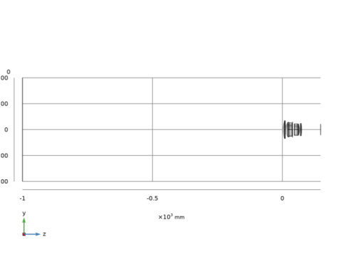
In the Application Libraries window, select Ray Optics Module>Lenses Cameras and Telescopes>double_gauss_lens in the tree.
|
|
3
|
Click
|
|
1
|
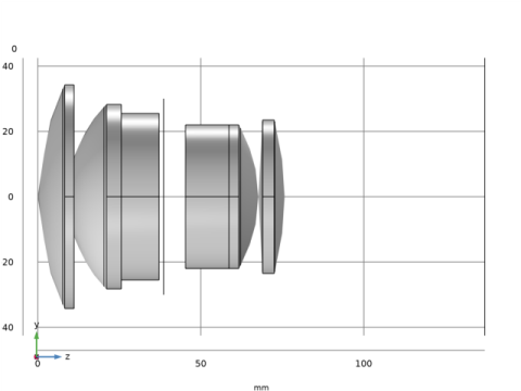
In the Model Builder window, expand the Component 1 (comp1)>Double Gauss Lens node, then click Stop (pi4).
|
|
2
|
|
1
|
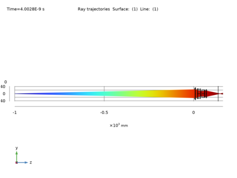
In the Model Builder window, under Component 1 (comp1) right-click Geometrical Optics (gop) and choose Release from Grid. This will be used to release rays from the object plane.
|
|
2
|
|
3
|
|
4
|
|
5
|
|
6
|
|
7
|
Specify the r vector as
|
|
8
|
In the α text field, type 0.70*atan(0.5*d1_clear_1/1[m]). This is the approximate angular size of the Double Gauss Lens entrance pupil as seen from the object plane.
|
|
1
|
|
2
|
|
3
|
In the Lengths text field, type 0 1200. The maximum optical path length now accounts for the distance to the object plane.
|
|
4
|
Locate the Physics and Variables Selection section. Select the Modify model configuration for study step check box.
|
|
5
|
In the tree, select Component 1 (Comp1)>Geometrical Optics (Gop)>Release from Grid 1 and Component 1 (Comp1)>Geometrical Optics (Gop)>Image.
|
|
6
|
Right-click and choose Disable. This disables the original (infinite conjugate) release. It also allows the rays to pass through the image plane which needs to be repositioned.
|
|
7
|
|
1
|
|
2
|
|
3
|
|
4
|
|
1
|
|
2
|
|
3
|
|
4
|
|
1
|
|
2
|
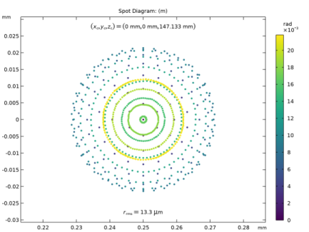
Right-click Spot Diagram 1 and choose Disable. This spot diagram is no longer used in this modified study.
|
|
1
|
|
2
|
|
3
|
|
4
|
Click to expand the Focal Plane Orientation section. Click Recompute Focal Plane Dataset. The Intersection Point Dataset will be repositioned to minimize the RMS spot size.
|
|
1
|
|
2
|
|
3
|
|
4
|
|
1
|
|
2
|
|
1
|
|
2
|
|
3
|
|
1
|
|
2
|
|
3
|
Locate the Parameters section. In the table, enter the following settings:
|
|
4
|
In the Model Builder window, under Global Definitions right-click Geometry Parts and choose Part Libraries.
|
|
1
|
In the Part Libraries window, select Ray Optics Module>3D>Apertures and Obstructions>rectangular_planar_annulus in the tree.
|
|
2
|
|
1
|
|
2
|
|
3
|
From the Part list, choose Rectangular Planar Annulus. This will convert the image plane from circular to rectangular.
|
|
4
|
|
5
|
Locate the Position and Orientation of Output section. Find the Coordinate system to match subsection. From the Take work plane from list, choose Lens 1 (pi1).
|
|
6
|
|
7
|
Find the Displacement subsection. In the zw text field, type Z_focus. This is the z-component of the best focus position.
|
|
1
|
In the Geometry toolbar, click
|
|
2
|
|
3
|
|
4
|
Locate the Position and Orientation of Output section. Find the Coordinate system to match subsection. From the Take work plane from list, choose Lens 1 (pi1).
|
|
5
|
|
6
|
|
7
|
|
8
|
|
9
|
|
10
|
Click OK.
|
|
11
|
|
1
|
|
2
|
|
3
|
|
4
|
|
5
|
|
6
|
|
1
|
|
2
|
|
3
|
From the Predefined list, choose Extra fine. It is necessary to increase the level of the Physics-based mesh refinement to account for the increase in size of the model geometry.
|
|
1
|
In the Mesh toolbar, click
|
|
2
|
|
3
|
|
1
|
|
3
|
|
4
|
In the Number of elements text field, type 2*npix. This ensures that there are approximately two mesh elements (in each direction) on the object plane for each image mesh element.
|
|
1
|
|
2
|
|
3
|
|
1
|
|
3
|
|
4
|
|
1
|
|
2
|
|
1
|
|
2
|
|
3
|
Click
|
|
4
|
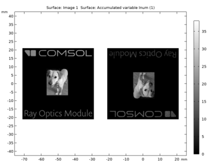
Browse to the model’s Application Libraries folder and double-click the file double_gauss_lens_image_simulation_example.png.
|
|
5
|
|
6
|
|
7
|
|
8
|
|
9
|
|
1
|
|
2
|
|
3
|
From the Selection list, choose Object Plane. This is the Boundary Selection referenced in the geometry Part Instance that defines the object plane.
|
|
4
|
|
5
|
|
6
|
In the ρ text field, type comp1.im1(x,y). The number density of the rays launched from the object plane will be proportional to the value of the image at each launch location.
|
|
7
|
|
8
|
|
9
|
Specify the r vector as
|
|
10
|
In the α text field, type 0.70*atan(0.5*d1_clear_1/abs(z)). The release angle is defined so that the entrance pupil is slightly overfilled.
|
|
11
|
From the Sampling from distribution list, choose Random. A random distribution ensures the entrance pupil is well sampled.
|
|
1
|
In the Physics toolbar, click
|
|
2
|
|
3
|
|
4
|
|
5
|
|
6
|
In the R text field, type 1. In this monochromatic simulation, each time a ray hits the image plane it is summed to create the final image.
|
|
1
|
|
2
|
|
3
|
In the tree, select Component 1 (Comp1)>Geometrical Optics (Gop)>Release from Boundary 1. This release is not used in the existing study.
|
|
4
|
Right-click and choose Disable.
|
|
1
|
|
2
|
|
3
|
Find the Studies subsection. In the Select Study tree, select Preset Studies for Selected Physics Interfaces>Ray Tracing.
|
|
4
|
|
5
|
|
1
|
|
2
|
|
3
|
Clear the Generate default plots check box. Because an image simulation may involve a large number of rays, some plots may need to adjusted manually.
|
|
1
|
|
2
|
|
3
|
|
4
|
|
5
|
|
6
|
Locate the Physics and Variables Selection section. Select the Modify model configuration for study step check box.
|
|
7
|
In the tree, select Component 1 (Comp1)>Geometrical Optics (Gop)>Release from Grid 1 and Component 1 (Comp1)>Geometrical Optics (Gop)>Release from Grid 2.
|
|
8
|
Right-click and choose Disable. These features are only used in Study 1.
|
|
1
|
|
2
|
|
3
|
Select the Only plot when requested check box. This is to avoid rendering an unnecessarily large number of rays used in an image simulation.
|
|
4
|
|
1
|
|
2
|
|
3
|
|
4
|
From the Solution list, choose Solution 2 (sol2). This creates a second Ray dataset based on the solution to the new study.
|
|
1
|
|
2
|
|
3
|
|
4
|
|
1
|
|
2
|
|
3
|
|
4
|
|
1
|
|
2
|
|
3
|
|
1
|
|
2
|
|
3
|
|
4
|
Click to expand the Window Settings section. Locate the Plot Settings section. From the View list, choose New view.
|
|
5
|
|
1
|
|
2
|
|
3
|
In the Maximum number of extra time steps text field, type 25. This will speed up the rendering of the rays.
|
|
1
|
|
2
|
|
3
|
In the Expression text field, type at(0,im1(qx,qy)). This will color each ray according to the value of the imported bitmap at location it was released.
|
|
4
|
|
1
|
|
2
|
|
3
|
|
4
|
|
1
|
In the Model Builder window, expand the Results>Ray Diagram 3>Surface 1 node, then click Selection 1.
|
|
2
|
|
3
|
|
1
|
|
2
|
|
3
|
|
4
|
Locate the Expression section. In the Expression text field, type im1(x,y). This will show the imported bitmap on the object plane.
|
|
5
|
|
6
|
|
7
|
|
1
|
|
2
|
|
3
|
|
4
|
Locate the Expression section. In the Expression text field, type gop.wall3.bacc1.Inum. This is the value of the accumulated image.
|
|
5
|
|
6
|
|
7
|
|
1
|
|
2
|
|
3
|
|
1
|
|
2
|
|
3
|
|
1
|
|
2
|
|
3
|
Locate the Data section. From the Dataset list, choose Image Surface. Note that this is actually the Image surface dataset.
|
|
4
|
Locate the Expression section. In the Expression text field, type im1(mag*x,mag*y). This scales and flips the object to match the image.
|
|
5
|
|
6
|
|
7
|
|
8
|
|
1
|
|
2
|
|
3
|
|
4
|
|
1
|
|
2
|
|
3
|
|
4
|
|
5
|
|
6
|
|
7
|
|
8
|