Fast Modeling of a Transmission Line Wilkinson Power Divider

Some conventional three-port power dividers are resistive power dividers and T-junction power dividers. Such dividers are either lossy or not matched to the system reference impedance at all ports. In addition, isolation between two coupled ports is not guaranteed. The Wilkinson power divider outperforms the lossless T-junction divider and the resistive divider and does not have the abovementioned issues. This example model simulates a Wilkinson power divider using the Transmission Line physics interface in 2D. This approach is very fast compared to solving Maxwell’s equations in 3D. The results present the S-parameters from 1 GHz to 5 GHz and electric potential distribution along the transmission line.

Figure 1: A microstrip Wilkinson power divider is composed of a 100 W resistor and transmission lines with two impedance values.

Model Definition

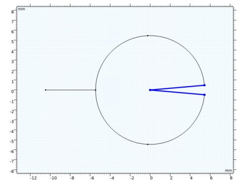
The power divider geometry consists of three straight lines built with Bézier polygons and three curved lines created by circles. Transmission Line Equation features define the distributed parameter values for 50 Ω and 70.71 Ω microstrip lines and it also defines the parameter values for the 100 Ω resistor connecting two 70.71 Ω microstrip lines.

The transmission line parameters for a 50 Ω microstrip line built on a 20 mil substrate with permittivity εr = 3.38 and 1 oz copper can be calculated accurately from Ref. 2.

Table 1: Calculated transmission line parameters of a 50 Ω microstrip line.
R	L	G	C
12.41 Ω/m	272.9 nH/m	0 S/m	107.1 pF/m

The contribution of the distributed resistance to the insertion loss with the given substrate properties is less than 0.05 dB. To make the modeling steps simpler in this example, the approximated parameter values in Table 2 are used for a 50 Ω microstrip line.

Table 2: simplified transmission line parameters of a 50 Ω microstrip line.
R	L	G	C
0 Ω/m	250 nH/m	0 S/m	100 pF/m

70.71 Ω microstrip line parameters are adjusted using the normalized impedance. The distributed inductance is proportionally scaled and the distributed capacitance is inversely scaled by the normalized impedance of the microstrip line. The distributed resistance for the 100 Ω resistor that connects two 70.71 Ω microstrip lines is scaled inversely by the length of the curvature where the resistor is placed.

In order to have a complete S-parameter report, port sweep option in the physics interface needs to be activated. When the port sweep is combined with a parametric sweep, this will excite ports one by one to generate a full S-parameter matrix plot.

Results and Discussion

In Figure 2 and Figure 3, the electric potential along the transmission lines are plotted. When port 3 ix excited, the input electric potential is not delivered to port 2 (Figure 2). Since the device is symmetric with regard to port 2 and 3, the isolation from port 2 to port 3 is also expected when port 2 is excited. This ensures two coupled ports (port 2 and port 3) are isolated from each other. When port 1 is excited, the input electric potential is split equally between port 2 and port 3 (Figure 3).

Figure 4 and Figure 5 show the computed S-parameter plots when port 1 and port 2 is excited, respectively. When the input power is equally split to two coupled ports, the received power level is -3 dB (S21 and S31) in each coupled port at 3 GHz. The impedance matching (S11 and S22) to the reference characteristic impedance 50 Ω and isolation (S23) are below -50 dB at the center frequency.

Figure 2: Port 3 is isolated from port 2 when port 3 is excited.

Figure 3: The input voltage is distributed equally between port 2 and port 3 when port 1 is excited.

Figure 4: The computed S-parameter plot when port 1 is excited.

Figure 5: The computed S-parameter plot when port 2 is excited.

References

1. D.M. Pozar, Microwave Engineering, John Wiley & Sons, 1998.

2. COMSOL Application Gallery, “Transmission Line Parameter Calculator”, https://www.comsol.com/model/transmission-line-parameter-calculator-22351

RF_Module/Couplers_and_Power_Dividers/transmission_line_wpd

Model Instructions

From the menu, choose .

New

In the window, click

Model Wizard

In the window, click

In the tree, select .

Click .

Click

In the tree, select .

Click

Global Definitions

Parameters 1

In the window, under click .

In the window for , locate the section.

In the table, enter the following settings:


Name	Expression	Value	Description
f0	3[GHz]	3E9 Hz	Center frequency
l0	250[nH/m]	2.5E-7 H/m	Distributed inductance, 50[ohm] line
c0	100[pF/m]	1E-10 F/m	Distributed capacitance, 50[ohm] line
z0	sqrt(l0/c0)	50 Ω	Characteristic impedance
lda0_t	1/f0/sqrt(l0*c0)	0.066667 m	Wavelength, transmission line
l1	l0*sqrt(2)	3.5355E-7 H/m	Distributed inductance, 70.71[ohm] line
c1	c0/sqrt(2)	7.0711E-11 F/m	Distributed capacitance, 70.71[ohm] line
z1	sqrt(l1/c1)	70.711 Ω	Characteristic impedance
r0	lda0_t/(4pi)360/350	0.0054567 m	Radius, 70.71[ohm] line

Geometry 1

In the window, under click .

In the window for , locate the section.

From the list, choose .

Line Segment 1 (ls1)

In the toolbar, click

and choose .

In the window for , locate the section.

From the list, choose .

Locate the section. From the list, choose .

Locate the section. In the text field, type -r0-5.

Locate the section. In the text field, type -r0.

Circle 1 (c1)

In the toolbar, click

In the window for , locate the section.

From the list, choose .

Locate the section. In the text field, type r0.

In the text field, type 350.

Locate the section. In the text field, type 5.

Click

Click the

button in the toolbar.

Delete Entities 1 (del1)

In the window, right-click and choose .

On the object , select Boundaries 5 and 6 only.

It might be easier to select the boundaries by using the window. To open this window, in the toolbar click and choose . (If you are running the cross-platform desktop, you find in the main menu.)

Delete total four line entities.

Circular Arc 1 (ca1)

In the toolbar, click

and choose .

In the window for , locate the section.

In the text field, type r0.

Locate the section. In the text field, type 355.

In the text field, type 5.

Line Segment 2 (ls2)

In the toolbar, click

and choose .

In the window for , locate the section.

From the list, choose .

Locate the section. From the list, choose .

Locate the section. In the text field, type r0*cos(5[deg]) .

In the text field, type r0*sin(5[deg]).

Locate the section. In the text field, type r0*2 .

In the text field, type r0.

Line Segment 3 (ls3)

In the toolbar, click

and choose .

In the window for , locate the section.

From the list, choose .

Locate the section. From the list, choose .

Locate the section. In the text field, type r0*cos(5[deg]).

In the text field, type -r0*sin(5[deg]).

Locate the section. In the text field, type r0*2.

In the text field, type -r0.

Click

Click the

button in the toolbar.

Transmission Line (tl)

Lumped Port 1

In the window, under right-click and choose .

Select Point 1 only.

Lumped Port 2

In the toolbar, click

and choose .

Select Point 8 only.

Lumped Port 3

In the toolbar, click

and choose .

Select Point 7 only.

Transmission Line Equation 1

Set parameter values for 50 Ω transmission lines. Since this is a default feature, the properties are applied to all line parts.

In the window, click .

In the window for , locate the section.

In the L text field, type l0.

In the C text field, type c0.

Transmission Line Equation 2

In the toolbar, click

and choose .

Select Boundaries 4–7 only.

Set parameter values for 70.71 Ω transmission lines. This overrides the default properties in the selected boundaries.

In the window for , locate the section.

In the L text field, type l1.

In the C text field, type c1.

Transmission Line Equation 3

In the toolbar, click

and choose .

Select Boundary 8 only.

In the toolbar, click

Check the Messages window to obtain the measured curvature length and use it to scale the distributed resistance. The transmission line with the adjusted resistance represents a 100 Ω resistor.

In the window for , locate the section.

In the R text field, type 100/0.9524e-3.

In the L text field, type 0.

In the C text field, type 0.

In the window, click .

In the window for , locate the section.

Select the check box.

Click . By clicking the button, all necessary port sweep settings such as sweep parameter and parametric study step will be automatically added. It is necessary to run the parametric sweep with port names to get a full S-parameter matrix.

Study 1

Step 1: Frequency Domain