PDF

Computing the Radar Cross Section of a Perfectly Conducting Sphere
General Description
This classic benchmark problem in computational electromagnetics is about computing the monostatic radar cross section (RCS) of a perfectly conducting sphere in free space, illuminated by a linearly polarized plane wave. The RCS is computed for sphere radius to free space wavelength ratios ranging from 0.1 to 0.8 and is compared to an exact analytical solution. This region represents the lower half of a transition zone between a long wavelength asymptotic solution, “Rayleigh scattering,” and a short wavelength asymptotic solution, “Geometrical Optics.” The transition zone is known as the “Mie region” after the originator of the exact solution. A mesh convergence study is performed for the first scattering resonance at a sphere radius to free space wavelength ratio of approximately 0.16364.
Model Setup
Geometry
Due to symmetry, it is sufficient to model only one quarter of the sphere. Figure 1 shows the geometry and boundary conditions.
Figure 1: The computational domain for computing the RCS of a PEC sphere in free space. Due to symmetry, it is sufficient to model one quarter of the sphere.
The geometry consists of two concentric spherical shells. The innermost shell, adjacent to the sphere, represents the free space domain, and the second shell represents a perfectly matched layer (PML) region that is used to provide an approximately reflection free termination of the, in reality unbounded, free space domain.
Equation
The model is set up and solved using a frequency domain formulation for the scattered electric field. The incident plane wave travels in the positive x direction, with the electric field polarized along the z-axis. The governing frequency domain equation can be written in the form
where the scattered electric field Esc is the dependent variable and the incident electric field Ei(0,0,Ez), with
The equation is discretized using second order edge elements (also known as vector elements, Nedelec elements, or curl-conforming elements). It is well known that in order to resolve the wave field, one should strive for 10 or more discretization points per wavelength. The combination of using second-order elements and 8 elements per wavelength fulfills this criterion with some margin. To respect the geometry, a mesh that is somewhat finer for the longest wavelengths is required on the surface of the scatterer. A maximum element size of half the radius is used on those boundaries. The PML region requires special meshing as described under the section Perfectly Matched Layer below.
Boundary conditions
The sphere has perfect electric conductor (PEC) boundaries. The PEC boundary condition
sets the tangential component of the electric field to zero. It is used for the modeling of lossless metallic surfaces or as a symmetry type boundary condition. It imposes symmetry for magnetic fields and “magnetic currents” and antisymmetry for electric fields and electric currents.
PEC boundary conditions and perfect magnetic conductor (PMC) boundary conditions apply on the symmetry planes used to subdivide the sphere model.
The PMC boundary condition
sets the tangential component of the magnetic field and thus also the surface current density to zero. On external boundaries, this can be interpreted as a “high surface impedance” boundary condition or used as a symmetry type boundary condition. It imposes symmetry for electric fields and electric currents and antisymmetry for magnetic fields and “magnetic currents.”
Perfectly Matched Layer
The PML region, the second concentric shell around the sphere, provides an approximately reflection free termination of the computational domain by applying a complex-valued coordinate stretching in the radial (outward) direction. For good accuracy, there should be at least five elements through the thickness of the PML. This condition is usually most efficiently met by using a swept mesh so that the effective element quality becomes insensitive to the scaling in the radial direction. The mesh used in this example is shown in Figure 2. It consists of a free tetrahedral mesh around the sphere and a swept mesh in the PML domain.
Figure 2: A free tetrahedral mesh is used in the free-space region around the sphere, and a swept mesh is used in the PML region.
The free space region around the sphere is defined to be the far-field domain. This specifies that a near-field to far-field calculation is done on the boundary of this domain, which takes the computed electric fields around the sphere and uses the Stratton-Chu equation to find the scattered electric field infinitely far away from the origin.
In 3D, this is:
For scattering problems, the far field in COMSOL is identical to what in physics is known as the “scattering amplitude.”
The radiating or scattering object is located in the vicinity of the origin, while the far-field point p is taken at infinity but with a well-defined angular position . 
In the above formulas,
E and H are the fields on the “aperture” — the surface S enclosing the sphere.
r0 is the unit vector pointing from the origin to the field point p. If the field points lie on a spherical surface S', r0 is the unit normal to S'.
n is the unit normal to the surface S.
η is the wave impedance:
k is the wave number.
λ is the wavelength.
r is the radius vector (not a unit vector) of the surface S.
Ep is the calculated far field in the direction from the origin toward point p.
The unit vector r0 can be interpreted as the direction defined by the angular position and Ep is the far field in this direction.
Results and Discussion
Figure 3 compares the simulation result for the RCS with the analytic solution computed using the scattered component of the electric field from this example and equation 11-247 in Ref. 1. As the figure shows, there is good agreement between the analytic solution determined in this manner and the finite-element model.
Figure 3: Comparison of the analytic solution and the COMSOL Multiphysics model of the RCS of a PEC sphere in free space.
Mesh Convergence
For the wavelength corresponding to the first maximum in the RCS plot in Figure 3, a mesh convergence study is performed to validate that the model converges toward a unique solution when refining the mesh isotropically. The model is solved in a parametric sweep over the number of mesh elements per wavelength. In the PML, the mesh density is not changed in the radial outward direction (that is, in the sweep direction for the swept mesh). The PML is resolved by 5 element layers in this direction which is sufficient to resolve the exponential damping in the radial direction. Thus the error contribution from the PML is not expected to decrease by adding more element layers. The main error contribution from the PML is due to the fact that it is not perfectly absorbing because of finite thickness and damping rather than mesh density. Thus, it is expected to give a contribution to the error in the computed RCS that does not decrease when refining the mesh.
Figure 4 shows the mesh convergence. The displayed error is the difference between the RCS from the finite element model and the exact solution from equation 11-247 in Ref. 1. As mentioned, the PML is expected to yield an error contribution which cannot be eliminated by refining the mesh. As there is no sign of stagnation in the convergence plot, this error contribution must be smaller than 0.1%. The RCS plot in Figure 3 corresponds to 8 elements per wavelength, that is a relative error of about 3% at the wavelength of the maximum in the RCS versus wavelength curve.
Figure 4: Mesh convergence for the difference in backscattering (monostatic) RCS between the COMSOL model and the exact solution.
Reference
1. C.A. Balanis, Advanced Engineering Electromagnetics, John Wiley & Sons, 1989.
Application Library path: RF_Module/Verification_Examples/rcs_sphere
Modeling Instructions
From the File menu, choose New.
New
In the New window, click  Model Wizard.
Model Wizard
1
In the Model Wizard window, click  3D.
2
In the Select Physics tree, select Radio Frequency>Electromagnetic Waves, Frequency Domain (emw).
3
Click Add.
4
Click  Study.
5
In the Select Study tree, select General Studies>Frequency Domain.
6
Global Definitions
Parameters 1
1
In the Model Builder window, under Global Definitions click Parameters 1.
2
In the Settings window for Parameters, locate the Parameters section.
3
Geometry 1
First, create a sphere with two layer definitions. The outermost layer represents the PMLs and the core represents the PEC sphere for RCS analysis. The median layer is the air domain.
Sphere 1 (sph1)
1
In the Geometry toolbar, click  Sphere.
2
In the Settings window for Sphere, locate the Size section.
3
In the Radius text field, type r0+t_air+t_pml.
4
Click to expand the Layers section. In the table, enter the following settings:
5
Click  Build All Objects.
Definitions
Add a view with a different angle of perspective.
View 2
In the Model Builder window, under Component 1 (comp1) right-click Definitions and choose View.
Camera
Change only the sign of y in the Position and Up Vector sections:
1
In the Model Builder window, expand the View 2 node, then click Camera.
2
In the Settings window for Camera, locate the Position section.
3
In the y text field, type 1.871.
4
Locate the Up Vector section. In the y text field, type -0.412.
5
Click  Update.
Choose wireframe rendering to get a better view of the interior parts.
6
Click the  Wireframe Rendering button in the Graphics toolbar.
Geometry 1
Due to the symmetry of the structure, it is sufficient to model only one quarter of the sphere. Delete the domains which are not part of the modeling domain.
Delete Entities 1 (del1)
1
In the Model Builder window, under Component 1 (comp1) right-click Geometry 1 and choose Delete Entities.
2
In the Settings window for Delete Entities, locate the Entities or Objects to Delete section.
3
From the Geometric entity level list, choose Domain.
4
On the object sph1, select Domains 1–3, 5–7, and 9–15 only.
5
Click  Build All Objects.
Definitions
View 1
After removing unnecessary domains, change the view to the first view definition which gives a better angle showing all layers.
1
Click the  Zoom Extents button in the Graphics toolbar.
This is the modeling domain for RCS analysis.
Electromagnetic Waves, Frequency Domain (emw)
Now set up the physics. You will solve the model for the scattered field, which requires background electric field (E-field) information. The background plane wave is traveling in the positive x direction, with the electric field polarized along the z-axis. The default boundary condition is perfect electric conductor, which applies to all exterior boundaries including the boundaries perpendicular to the background E-field polarization.
1
In the Model Builder window, under Component 1 (comp1) click Electromagnetic Waves, Frequency Domain (emw).
2
In the Settings window for Electromagnetic Waves, Frequency Domain, locate the Formulation section.
3
From the list, choose Scattered field.
4
Specify the Eb vector as
Choose wireframe rendering in the current view to get a better view of the interior parts.
5
Click the  Wireframe Rendering button in the Graphics toolbar.
Scattering Boundary Condition 1
1
In the Physics toolbar, click  Boundaries and choose Scattering Boundary Condition.
2
Definitions
The outermost domains from the center of the sphere are the PMLs.
Perfectly Matched Layer 1 (pml1)
1
In the Definitions toolbar, click  Perfectly Matched Layer.
2
3
In the Settings window for Perfectly Matched Layer, locate the Geometry section.
4
From the Type list, choose Spherical.
Electromagnetic Waves, Frequency Domain (emw)
Set PMC on the boundaries parallel to the background E-field polarization.
Perfect Magnetic Conductor 1
1
In the Physics toolbar, click  Boundaries and choose Perfect Magnetic Conductor.
2
Far-Field Domain 1
In the Physics toolbar, click  Domains and choose Far-Field Domain.
Far-Field Calculation 1
1
In the Model Builder window, expand the Far-Field Domain 1 node, then click Far-Field Calculation 1.
2
In the Settings window for Far-Field Calculation, locate the Far-Field Calculation section.
3
Select the Symmetry in the y=0 plane check box.
4
Select the Symmetry in the z=0 plane check box.
5
From the Symmetry type list, choose Symmetry in H (PEC).
Materials
Next, assign material properties. Use air for all domains.
Add Material
1
In the Home toolbar, click  Add Material to open the Add Material window.
2
Go to the Add Material window.
3
4
Click Add to Component in the window toolbar.
5
In the Home toolbar, click  Add Material to close the Add Material window.
Mesh 1
Use a tetrahedral mesh for the air domains.
Free Tetrahedral 1
1
In the Mesh toolbar, click  Free Tetrahedral.
2
In the Settings window for Free Tetrahedral, locate the Domain Selection section.
3
From the Geometric entity level list, choose Domain.
4
The maximum mesh size is at most 0.2 wavelengths in free space. In this model, use 0.125 wavelengths.
Size
1
In the Model Builder window, click Size.
2
In the Settings window for Size, locate the Element Size section.
3
Click the Custom button.
4
Locate the Element Size Parameters section. In the Maximum element size text field, type lda/h_size.
5
In the Minimum element size text field, type lda/h_size.
Use a swept mesh for the PML domains.
Swept 1
In the Mesh toolbar, click  Swept.
Distribution 1
1
Right-click Swept 1 and choose Distribution.
2
Right-click Distribution 1 and choose Build All.
Compare the mesh with that shown in Figure 2.
Study 1
Parametric Sweep
1
In the Study toolbar, click  Parametric Sweep.
2
In the Settings window for Parametric Sweep, locate the Study Settings section.
3
4
Step 1: Frequency Domain
1
In the Model Builder window, click Step 1: Frequency Domain.
2
In the Settings window for Frequency Domain, locate the Study Settings section.
3
In the Frequencies text field, type f0.
4
In the Model Builder window, click Study 1.
5
In the Settings window for Study, locate the Study Settings section.
6
Clear the Generate default plots check box.
7
In the Study toolbar, click  Compute.
Results
Follow the instructions below to reproduce the plot in Figure 3. First, show the computed RCS values using square markers.
1D Plot Group 1
1
In the Home toolbar, click  Add Plot Group and choose 1D Plot Group.
2
In the Settings window for 1D Plot Group, locate the Data section.
3
From the Dataset list, choose Study 1/Parametric Solutions 1 (sol2).
4
Click to expand the Title section. From the Title type list, choose Custom.
5
Find the Type and data subsection. Clear the Unit check box.
6
Clear the Description check box.
7
Clear the Type check box.
8
Find the User subsection. In the Prefix text field, type RCS Calculation.
9
Locate the Plot Settings section. Select the x-axis label check box.
10
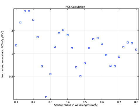
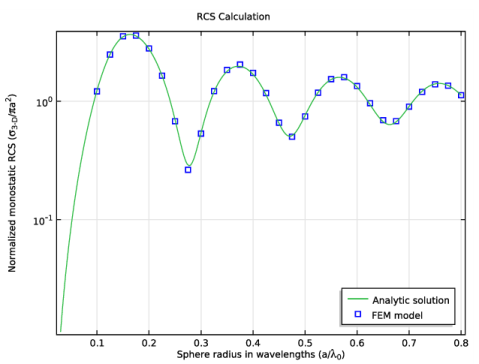
In the associated text field, type Sphere radius in wavelengths (a/\lambda<sub>0</sub>).
11
Select the y-axis label check box.
12
In the associated text field, type Normalized monostatic RCS (\sigma<sub>3-D</sub>/\pi a<sup>2</sup>).
13
Locate the Axis section. Select the y-axis log scale check box.
Point Graph 1
1
Right-click 1D Plot Group 1 and choose Point Graph.
2
3
In the Settings window for Point Graph, locate the y-Axis Data section.
4
In the Expression text field, type emw.bRCS3D/(pi*r0^2).
5
Locate the x-Axis Data section. From the Axis source data list, choose Outer solutions.
6
Click to expand the Coloring and Style section. Find the Line style subsection. From the Line list, choose None.
7
Find the Line markers subsection. From the Marker list, choose Square.
8
From the Positioning list, choose In data points.
9
In the 1D Plot Group 1 toolbar, click  Plot.
The observed RCS graph pattern is oscillatory in the Mie region.
Next, proceed to perform the mesh convergence study at the first resonance in the Mie region.
Start by extending the parameter list with the resonant radius and the associated theoretical RCS value.
Global Definitions
Parameters 1
Add the two rows at the end and change the first line according to.
1
In the Model Builder window, under Global Definitions click Parameters 1.
2
In the Settings window for Parameters, locate the Parameters section.
3
Mesh 1
Add a new mesh with some tweaks to make sure that the curvature of the sphere is always resolved.
This is to avoid inverted mesh elements.
1
In the Model Builder window, under Component 1 (comp1) right-click Mesh 1 and choose Duplicate.
Mesh 2
Size
1
In the Model Builder window, expand the Mesh 2 node, then click Size.
2
In the Settings window for Size, locate the Element Size Parameters section.
3
In the Minimum element size text field, type if(lda/h_size>r0/2,r0/2,lda/h_size).
Size 1
1
In the Model Builder window, right-click Free Tetrahedral 1 and choose Size.
2
In the Settings window for Size, locate the Geometric Entity Selection section.
3
From the Geometric entity level list, choose Boundary.
4
Click  Paste Selection.
5
In the Paste Selection dialog box, type 7,10 in the Selection text field.
6
7
In the Settings window for Size, locate the Element Size section.
8
Click the Custom button.
9
Locate the Element Size Parameters section. Select the Maximum element size check box.
10
In the associated text field, type if(lda/h_size>r0/2,r0/2,lda/h_size).
Root
Add a new frequency domain study for the mesh convergence analysis.
Add Study
1
In the Home toolbar, click  Add Study to open the Add Study window.
2
Go to the Add Study window.
3
Find the Studies subsection. In the Select Study tree, select General Studies>Frequency Domain.
4
Click Add Study in the window toolbar.
5
In the Home toolbar, click  Add Study to close the Add Study window.
Study 2
A parametric sweep is needed to loop over the mesh sizes.
Parametric Sweep
1
In the Study toolbar, click  Parametric Sweep.
2
In the Settings window for Parametric Sweep, locate the Study Settings section.
3
4
Step 1: Frequency Domain
1
In the Model Builder window, click Step 1: Frequency Domain.
2
In the Settings window for Frequency Domain, locate the Study Settings section.
3
In the Frequencies text field, type f0.
4
In the Model Builder window, click Study 2.
5
In the Settings window for Study, locate the Study Settings section.
6
Clear the Generate default plots check box.
7
In the Study toolbar, click  Compute.
Results
Continue to plot the relative error versus elements per wavelength.
1D Plot Group 2
1
In the Home toolbar, click  Add Plot Group and choose 1D Plot Group.
2
In the Settings window for 1D Plot Group, locate the Data section.
3
From the Dataset list, choose Study 2/Parametric Solutions 2 (sol33).
4
Locate the Plot Settings section. Select the x-axis label check box.
5
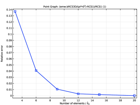
In the associated text field, type Number of elements / \lambda<sub>0</sub>.
6
Select the y-axis label check box.
7
Point Graph 1
1
Right-click 1D Plot Group 2 and choose Point Graph.
2
In the Settings window for Point Graph, locate the Selection section.
3
Click  Paste Selection.
4
In the Paste Selection dialog box, type 2 in the Selection text field.
5
6
In the Settings window for Point Graph, locate the y-Axis Data section.
7
In the Expression text field, type (emw.bRCS3D/(pi*r0^2)-RCS1)/RCS1.
8
Locate the x-Axis Data section. From the Axis source data list, choose h_size.
9
From the Parameter list, choose Expression.
10
In the Expression text field, type h_size.
11
Locate the Coloring and Style section. In the Width text field, type 2.
12
Find the Line markers subsection. From the Marker list, choose Square.
13
From the Positioning list, choose In data points.
14
Click the  x-Axis Log Scale button in the Graphics toolbar.
15
Click the  y-Axis Log Scale button in the Graphics toolbar.
16
In the 1D Plot Group 2 toolbar, click  Plot.
Compare the convergence plot with that shown in Figure 4.