PDF

Biconical Antenna
Introduction
The biconical antenna is a wideband antenna with an omnidirectional radiation pattern. This example models such an antenna, including its coaxial feed structure.
Figure 1: Biconical antenna fed by a coaxial lumped port. The region of free space around the antenna is truncated by a perfectly matched layer (PML).
Model Definition
The biconical antenna, shown in Figure 1, is composed of two conical, metallic, radiating elements. Figure 2 shows the details of the feed structure at the center. A short section of a dielectric-filled coaxial cable starts at a small cylindrical domain containing the power source, which is not part of the model domain. Instead, you model the source by applying a coaxial lumped port condition at the boundary facing the coaxial cable, which launches a wave down the coax. The inner and outer conductors of the coax are connected to the cone-shaped radiators via wires that you model as perfect electric conductors. A small symmetric cutout in each cone provides sufficient clearance for mounting and assembly. The distance between radiators and the surface area of the cone end tips controls the reactance of the antenna’s input port, and can be adjusted to alter antenna performance.
Figure 2: The zoomed view of the coaxial lumped port. The coaxial cable begins at a small cylindrical domain that is external to the model domain, as are the wire interiors.
Results and Discussion
The simulated results in Figure 3 shows that S11 is less than 10 dB from 1.5 GHz to 3.5 GHz. This is much wider than a typical dipole antenna bandwidth. The radiation pattern at the E-plane and the H-plane resembles that from a dipole antenna. The biconical antenna works well in applications requiring an omnidirectional radiation pattern and a wide bandwidth.
Figure 3: The frequency response of the biconical antenna shows wideband impedance matching.
Figure 4: Far-field radiation pattern at the E-plane (blue) and the H-plane (green) at 1.9 GHz. It is similar to the radiation pattern of a dipole antenna.
References
1. D.M. Pozar, Microwave Engineering, John Wiley & Sons, 1998.
2. C.A. Balanis, Antenna Theory, John Wiley & Sons, 1997.
3. R.E. Collin, Antennas and Radiowave Propagation, McGraw-Hill, 1985.
Application Library path: RF_Module/Antennas/biconical_antenna
Modeling Instructions
From the File menu, choose New.
New
In the New window, click  Model Wizard.
Model Wizard
1
In the Model Wizard window, click  3D.
2
In the Select Physics tree, select Radio Frequency>Electromagnetic Waves, Frequency Domain (emw).
3
Click Add.
4
Click  Study.
5
In the Select Study tree, select General Studies>Frequency Domain.
6
Study 1
Step 1: Frequency Domain
1
In the Model Builder window, under Study 1 click Step 1: Frequency Domain.
2
In the Settings window for Frequency Domain, locate the Study Settings section.
3
In the Frequencies text field, type range(1.5[GHz],0.2[GHz],3.5[GHz]).
Geometry 1
1
In the Model Builder window, under Component 1 (comp1) click Geometry 1.
2
In the Settings window for Geometry, locate the Units section.
3
From the Length unit list, choose mm.
First, add a cylinder for the inner conductor.
Cylinder 1 (cyl1)
1
In the Geometry toolbar, click  Cylinder.
2
In the Settings window for Cylinder, locate the Size and Shape section.
3
In the Radius text field, type 0.635.
4
In the Height text field, type 7.95.
5
Locate the Position section. In the x text field, type -10.
6
In the z text field, type 1.2.
7
Locate the Axis section. From the Axis type list, choose x-axis.
8
Click  Build Selected.
9
Click the  Wireframe Rendering button in the Graphics toolbar.
Add a concentric cylinder to include the outer conductor.
Cylinder 2 (cyl2)
1
In the Geometry toolbar, click  Cylinder.
2
In the Settings window for Cylinder, locate the Size and Shape section.
3
In the Radius text field, type 2.05.
4
In the Height text field, type 6.
5
Locate the Position section. In the x text field, type -10.
6
In the z text field, type 1.2.
7
Locate the Axis section. From the Axis type list, choose x-axis.
8
Click to expand the Layers section. In the table, enter the following settings:
9
Clear the Layers on side check box.
10
Select the Layers on bottom check box.
11
Click  Build Selected.
12
Click the  Zoom Extents button in the Graphics toolbar.
Next, create a structure connecting the coaxial cable and the radiator.
Torus 1 (tor1)
1
In the Geometry toolbar, click  Torus.
2
In the Settings window for Torus, locate the Size and Shape section.
3
In the Major radius text field, type 2.05.
4
In the Minor radius text field, type 0.635.
5
In the Revolution angle text field, type 90.
6
Locate the Position section. In the x text field, type -2.05.
7
In the z text field, type 2.25+1.
8
Locate the Axis section. From the Axis type list, choose Cartesian.
9
In the y text field, type 1.
10
In the z text field, type 0.
11
Locate the Rotation Angle section. In the Rotation text field, type 270.
12
Click  Build Selected.
Create a domain backing the lumped port. This part is excluded from the model space later on.
Cylinder 3 (cyl3)
1
In the Geometry toolbar, click  Cylinder.
2
In the Settings window for Cylinder, locate the Size and Shape section.
3
In the Radius text field, type 0.635.
4
In the Height text field, type 4.95.
5
Locate the Position section. In the x text field, type -7.
6
In the z text field, type -1.2.
7
Locate the Axis section. From the Axis type list, choose Cartesian.
8
In the x text field, type 1.
9
In the z text field, type 0.
10
Click  Build Selected.
Go on to add a radiator cone.
Cone 1 (cone1)
1
In the Geometry toolbar, click  Cone.
2
In the Settings window for Cone, locate the Size and Shape section.
3
In the Bottom radius text field, type 51.
4
In the Height text field, type 51.
5
From the Specify top size using list, choose Angle.
6
In the Semiangle text field, type 40.
7
Locate the Position section. In the z text field, type 54.25.
8
Locate the Axis section. From the Axis type list, choose Cartesian.
9
In the z text field, type -1.
10
Click  Build Selected.
Add a block representing the assembly and mounting cutout from the upper radiator.
Block 1 (blk1)
1
In the Geometry toolbar, click  Block.
2
In the Settings window for Block, locate the Size and Shape section.
3
In the Width text field, type 8.
4
In the Depth text field, type 9.
5
In the Height text field, type 3.
6
Locate the Position section. In the x text field, type -10.
7
In the y text field, type -4.5.
8
In the z text field, type 2.
9
Click  Build Selected.
Difference 1 (dif1)
1
In the Geometry toolbar, click  Booleans and Partitions and choose Difference.
2
3
In the Settings window for Difference, locate the Difference section.
4
Find the Objects to subtract subsection. Click to select the  Activate Selection toggle button.
5
6
Click  Build Selected.
Generate the second radiator by mirroring the first one.
Mirror 1 (mir1)
1
In the Geometry toolbar, click  Transforms and choose Mirror.
2
Select the objects dif1 and tor1 only.
3
In the Settings window for Mirror, locate the Input section.
4
Select the Keep input objects check box.
5
Click  Build Selected.
Sphere 1 (sph1)
1
In the Geometry toolbar, click  Sphere.
2
In the Settings window for Sphere, locate the Size section.
3
In the Radius text field, type 150.
4
Click to expand the Layers section. In the table, enter the following settings:
5
Click  Build All Objects.
6
Click the  Go to Default View button in the Graphics toolbar.
Definitions
External Domains
1
In the Definitions toolbar, click  Explicit.
Next, create a set of selections for use when setting up the physics.
2
In the Settings window for Explicit, type External Domains in the Label text field.
3
You can do this most easily by copying the text ’8, 9, 11, 12, and 14-16’, clicking in the selection box, and then pressing Ctrl+V, or by using the Paste Selection dialog box.
4
Click the  Go to Default View button in the Graphics toolbar.
Model Domains
1
In the Definitions toolbar, click  Complement.
2
In the Settings window for Complement, type Model Domains in the Label text field.
3
Locate the Input Entities section. Under Selections to invert, click  Add.
4
In the Add dialog box, select External Domains in the Selections to invert list.
5
Internal PEC Boundaries
1
In the Definitions toolbar, click  Explicit.
2
In the Settings window for Explicit, type Internal PEC Boundaries in the Label text field.
3
Locate the Input Entities section. From the Geometric entity level list, choose Boundary.
4
5
Click the  Zoom In button in the Graphics toolbar, a couple of times to see the selected boundaries clearly.
Perfectly Matched Layer 1 (pml1)
1
In the Definitions toolbar, click  Perfectly Matched Layer.
2
3
In the Settings window for Perfectly Matched Layer, locate the Geometry section.
4
From the Type list, choose Spherical.
Hide some domains to get a better view of the interior parts.
Hide for Physics 1
1
In the Model Builder window, right-click View 1 and choose Hide for Physics.
2
Electromagnetic Waves, Frequency Domain (emw)
1
In the Model Builder window, under Component 1 (comp1) click Electromagnetic Waves, Frequency Domain (emw).
2
In the Settings window for Electromagnetic Waves, Frequency Domain, locate the Domain Selection section.
3
From the Selection list, choose Model Domains.
Perfect Electric Conductor 2
1
In the Physics toolbar, click  Boundaries and choose Perfect Electric Conductor.
2
In the Settings window for Perfect Electric Conductor, locate the Boundary Selection section.
3
From the Selection list, choose Internal PEC Boundaries.
While the perfect electric conductor is the default boundary condition for exterior boundaries, you need to apply this condition explicitly to interior boundaries.
Lumped Port 1
1
In the Physics toolbar, click  Boundaries and choose Lumped Port.
2
3
In the Settings window for Lumped Port, locate the Lumped Port Properties section.
4
From the Type of lumped port list, choose Coaxial.
For the first port, wave excitation is on by default.
Far-Field Domain 1
In the Physics toolbar, click  Domains and choose Far-Field Domain.
Add Material
1
In the Home toolbar, click  Add Material to open the Add Material window.
2
Go to the Add Material window.
3
4
Click Add to Component in the window toolbar.
5
In the Home toolbar, click  Add Material to close the Add Material window.
Materials
Air (mat1)
Override this material for the coaxial cable domain.
PTFE
1
In the Model Builder window, right-click Materials and choose Blank Material.
2
In the Settings window for Material, type PTFE in the Label text field.
3
4
Locate the Material Contents section. In the table, enter the following settings:
Mesh 1
1
In the Model Builder window, under Component 1 (comp1) click Mesh 1.
2
In the Settings window for Mesh, locate the Physics-Controlled Mesh section.
3
From the Element size list, choose Fine.
4
Click  Build All.
5
Click the  Zoom Extents button in the Graphics toolbar.
6
Click the  Zoom In button in the Graphics toolbar.
7
Click the  Reset Hiding button in the Graphics toolbar, to reset the visibility state of the hidden domains in preparation of the results processing.
Study 1
In the Home toolbar, click  Compute.
Results
Electric Field (emw)
Begin the results analysis and visualization by modifying the first default plot to show the E-field norm in the xz-plane.
Multislice
1
In the Model Builder window, expand the Electric Field (emw) node, then click Multislice.
2
In the Settings window for Multislice, locate the Expression section.
3
In the Expression text field, type 20*log10(emw.normE).
4
Select the Description check box.
5
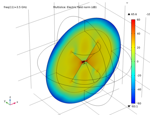
In the associated text field, type Electric field norm (dB).
6
Locate the Multiplane Data section. Find the Z-planes subsection. In the Planes text field, type 0.
7
Find the X-planes subsection. In the Planes text field, type 0.
8
Click to expand the Range section. Select the Manual color range check box.
9
In the Minimum text field, type -60.
10
In the Maximum text field, type 60.
11
In the Electric Field (emw) toolbar, click  Plot.
Use the zoom controls in the Graphics toolbar to explore the plot further.
The following instructions reproduce the frequency-response plot shown in Figure 3.
Smith Plot (emw)
3D Far Field, Gain (emw)
1
In the Model Builder window, click 3D Far Field, Gain (emw).
2
In the Settings window for 3D Plot Group, locate the Data section.
3
From the Parameter value (freq (GHz)) list, choose 1.5.
4
In the 3D Far Field, Gain (emw) toolbar, click  Plot.
3D far-field pattern is isotropic on the xy-plane.
Finally, reproduce the polar plot of the far-field on the E- and H-plane.
Polar Plot Group 6
1
In the Home toolbar, click  Add Plot Group and choose Polar Plot Group.
2
In the Settings window for Polar Plot Group, locate the Data section.
3
From the Parameter selection (freq) list, choose From list.
4
In the Parameter values (freq (GHz)) list, select 1.9.
Radiation Pattern 1
1
In the Polar Plot Group 6 toolbar, click  More Plots and choose Radiation Pattern.
2
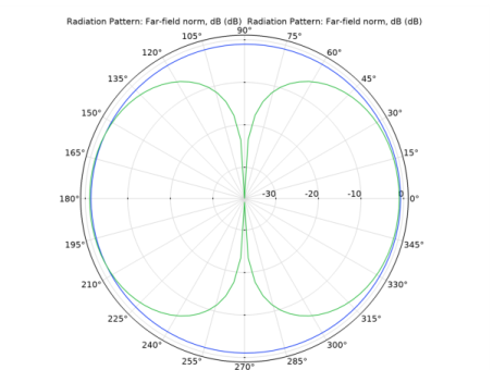
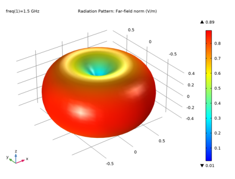
In the Settings window for Radiation Pattern, click Replace Expression in the upper-right corner of the Expression section. From the menu, choose Component 1 (comp1)>Electromagnetic Waves, Frequency Domain>Far field>emw.normdBEfar - Far-field norm, dB - dB.
3
Locate the Evaluation section. Find the Angles subsection. In the Number of angles text field, type 100.
Radiation Pattern 2
1
Right-click Radiation Pattern 1 and choose Duplicate.
2
In the Settings window for Radiation Pattern, locate the Evaluation section.
3
Find the Reference direction subsection. In the x text field, type 0.
4
In the y text field, type 1.
5
Find the Normal vector subsection. In the x text field, type 1.
6
In the z text field, type 0.
7
In the Polar Plot Group 6 toolbar, click  Plot.
Compare the resulting plot with that shown in Figure 4.