PDF

Behavior of a Power-Law Fluid in a Mixer
Introduction
Mixers are often used to process non-Newtonian fluids and many of those fluids can be modeled using a power law for the relation between viscosity and shear rate. This model simulates the flow in a flat-bottom tank with a single four-blade pitched impeller. The simulated fluid is a solution of 1% Carbopol in water, which is a shear-thinning fluid that can be modeled by the power law. The calculated power numbers are compared with experimental results.
General Description
Geometry
The model is one of the cases considered in Ref. 1. The complete model geometry is shown in Figure 1. It is a flat bottom tank with diameter T = 0.45 m and height H = 0.44 m. It has four baffles with width W = 1/12·T. In the tank, there is an impeller which in Ref. 1 is specified to be an A200 impeller (Ref. 2). That means, that the impeller is a four-blade impeller with flat, 45° pitched blades. The impeller diameter, Da, is 0.41·T and the clearance (the distance between the bottom of the tank and the impeller), C, is 0.75·Da.
Figure 1: Flat-bottom tank with a four-blade, pitched impeller.
Liquid
The liquid is a 0.1 % Carbopol solution in water. It is a shear-thinning fluid and was selected in Ref. 1 since it is transparent enough for laser Doppler velocimetry. Rheological measurements suggest that the solution can be modeled as a power-law fluid under the range of shear rates expected in this set-up. The power law prescribes the following relation between the viscous stress K and the strain rate tensor S
(1)
where is the shear rate, m is the power-law consistency coefficient and n is the flow-behavior index. According to Ref. 1, for shear rates in the range of 0.1–1000 s1, m = 9 and n = 0.2.
Reynolds Number and Power Number
This model computes the power number, Np, as a function of the impeller Reynolds number, NRe.
The power number is defined by (Ref. 3)
where ρ is the fluid density, N is the rotations per second, Da is the impeller diameter and P is the power draw which in turn is determined by
(2)
In Equation 2, the integral is taken over the surface of the impeller. Ω is the rotational speed vector and Γ is the torque acting on a point r = {x, y, z} is defined by
where F is the force acting on each point of the surface.
For a Newtonian fluid, the impeller Reynolds number is defined as
(3)
where μ is the (Newtonian) dynamic viscosity. Equation 3 is however not valid for a shear-thinning liquid where the viscosity may vary by several order of magnitudes throughout the model. In the laminar flow regime, the impeller Reynolds number is instead calculated using the Metzner and Otto method (Ref. 1 and Ref. 3) where the viscosity μ is replaced by an average, near-impeller viscosity, μavg, defined by
(4)
where m is the power-law consistency coefficient and n is the flow-behavior index. in Equation 4 is an average, near-impeller shear rate that can be calculated as a function of the impeller rotational speed:
(5)
where Ks is a constant that is assumed to depend only on impeller geometry. For the A200 impeller, Ks = 8.58 (Ref. 1). Combining Equation 3, Equation 4, and Equation 5 gives
In this model, the Reynolds number NRe = 50, 100, 200, and 400 which corresponds to N = 1.6337, 2.4001, 3.529, and 5.187 respectively.
Model Setup
A fully correct flow pattern can be obtained from a time-dependent simulation of the complete geometry shown in Figure 1. This would however be a very time-consuming procedure. Ref. 1 therefore uses a method equivalent to the frozen-rotor approach available in COMSOL. In a frozen-rotor approach, the impeller does not actually rotate. Instead, the rotational effect is included by the means of Coriolis and centrifugal forces. With a frozen-rotor approach, it is possible to utilize the symmetry of the geometry and only solve for a quarter of the mixer as shown in Figure 2. The geometry can be seen to have two domains. The domain enclosing the impeller is specified as rotating while the outer domain is stationary. This decomposition is not necessary when using a frozen-rotor approach, but it simplifies the setup of the boundary conditions.
Figure 2: Geometry used in the simulation.
Both baffles and impeller blades are very thin and are therefore treated as walls with zero thickness. This is a reasonable assumption for axial impellers (Ref. 4).
The power law (Equation 1) predicts infinite effective viscosity at zero shear rate, which of course is non-physical. The power law is therefore supplemented with a lower limit on the shear rate, . In this model, is set to 0.1 s1 which is the lowest shear rate for which the power law is a valid viscosity model for the Carbopol solution.
To calculate the power, notice that, since the impeller shaft is parallel to the z-axis, Ω has only one component and is equal to {0, 0, 2πN}. This means that Equation 2 reduces to
(6)
Results and Discussion
Figure 3 shows the flow pattern for NRe = 400. Fluid is ejected downward from the impeller and is recirculated back along the outer wall. The movement of the fluid is almost entirely restricted to a high-shear region close to the impeller where the viscosity is low. The effective viscosity in the rest of the mixer is very high and the fluid there behaves more like a solid. The logarithm of the effective viscosity is shown in Figure 4.
Figure 3: Velocity vectors and velocity magnitude for NRe = 400.
Figure 4: Logarithm of the effective viscosity for NRe = 400. Arrows show the velocity field.
The calculated power numbers are plotted in Figure 5 together with the experimental results from Ref. 1. The agreement is at least as good as the agreement between experiments and simulations reported in Ref. 1.
Figure 5: Power number as a function of Reynolds number.
References
1. W. Kelly and B. Gigas, “Using CFD to predict the behavior of power law fluids near axial-flow impellers operating in the transitional flow regime,” Chem. Eng. Science, vol. 58, pp. 2141–2152, 2003.
2. SPX Lightnin A200 impeller, http://www.spx.com/en/lightnin/pc-impellers/
3. E.L. Paul, V.A. Atiemo-Obeng, and S.M. Dresta, eds., Handbook of Industrial Mixing, Science and Practice, John Wiley & Sons, 2004.
4. D. Chapple, S.M. Kresta, A. Wall, and A. Afacan, “The Effect of Impeller and Tank Geometry on Power Number for a pitched blade Turbine,” Trans IChemE, vol. 80, pp. 364–372, 2002.
Application Library path: Polymer_Flow_Module/Verification_Examples/power_law_mixer
Modeling Instructions
From the File menu, choose New.
New
In the New window, click  Model Wizard.
Model Wizard
1
In the Model Wizard window, click  3D.
2
In the Select Physics tree, select Fluid Flow>Single-Phase Flow>Rotating Machinery, Fluid Flow>Laminar Flow.
3
Click Add.
4
Click  Study.
5
In the Select Study tree, select Preset Studies for Selected Physics Interfaces>Frozen Rotor.
6
Load the geometry sequence from file. Note that parameters used in the geometry are included with the sequence.
Geometry 1
1
In the Geometry toolbar, click Insert Sequence and choose Insert Sequence.
2
3
In the Geometry toolbar, click  Build All.
Also load parameters for the fluid properties and the simulation conditions.
Global Definitions
Parameters 1
1
In the Model Builder window, under Global Definitions click Parameters 1.
2
In the Settings window for Parameters, locate the Parameters section.
3
Click  Load from File.
4
Moving Mesh
Rotating Domain 1
1
In the Model Builder window, under Component 1 (comp1)>Moving Mesh click Rotating Domain 1.
2
3
In the Settings window for Rotating Domain, locate the Rotation section.
4
In the f text field, type -N0.
Materials
Add blank materials for the fluid. You will specify the fluid properties after the setup of the physics interface.
Material 1 (mat1)
In the Model Builder window, under Component 1 (comp1) right-click Materials and choose Blank Material.
Laminar Flow (spf)
Fluid Properties 1
1
In the Settings window for Fluid Properties, locate the Fluid Properties section.
2
Find the Constitutive relation subsection. From the list, choose Inelastic non-Newtonian.
3
From the Inelastic model list, choose Power law.
Now, COMSOL recognizes which material properties are required to solve this model.
Materials
Material 1 (mat1)
1
In the Model Builder window, under Component 1 (comp1)>Materials click Material 1 (mat1).
2
In the Settings window for Material, locate the Material Contents section.
3
Laminar Flow (spf)
Fluid Properties 1
Increase the lower shear rate limit.
1
In the Model Builder window, under Component 1 (comp1)>Laminar Flow (spf) click Fluid Properties 1.
2
Interior Wall 1
1
In the Physics toolbar, click  Boundaries and choose Interior Wall.
2
In the Settings window for Interior Wall, locate the Boundary Selection section.
3
From the Selection list, choose Rotating Interior Wall.
Interior Wall 2
1
In the Physics toolbar, click  Boundaries and choose Interior Wall.
2
In the Settings window for Interior Wall, locate the Boundary Selection section.
3
From the Selection list, choose Interior Wall.
Symmetry 1
1
In the Physics toolbar, click  Boundaries and choose Symmetry.
2
In the Settings window for Symmetry, locate the Boundary Selection section.
3
From the Selection list, choose Symmetry.
Periodic Flow Condition 1
1
In the Physics toolbar, click  Boundaries and choose Periodic Flow Condition.
2
Pressure Point Constraint 1
1
In the Physics toolbar, click  Points and choose Pressure Point Constraint.
2
In the Settings window for Pressure Point Constraint, locate the Point Selection section.
3
From the Selection list, choose Fixed point (Flat Bottom Tank 1).
Mesh 1
Size
1
In the Model Builder window, under Component 1 (comp1) right-click Mesh 1 and choose Edit Physics-Induced Sequence.
2
In the Settings window for Size, locate the Element Size section.
3
From the Predefined list, choose Normal.
Size 1
1
In the Model Builder window, expand the Size node, then click Component 1 (comp1)>Mesh 1>Size 1.
2
In the Settings window for Size, locate the Element Size section.
3
From the Predefined list, choose Finer.
Size 2
1
In the Model Builder window, right-click Mesh 1 and choose Size.
2
In the Settings window for Size, locate the Geometric Entity Selection section.
3
From the Geometric entity level list, choose Boundary.
4
From the Selection list, choose Rotating Interior Wall.
5
Locate the Element Size section. From the Calibrate for list, choose Fluid dynamics.
6
From the Predefined list, choose Extra fine.
7
Right-click Size 2 and choose Move Up.
8
Right-click Size 2 and choose Move Up.
9
Right-click Size 2 and choose Move Up.
Size 3
1
In the Model Builder window, right-click Mesh 1 and choose Size.
2
In the Settings window for Size, locate the Geometric Entity Selection section.
3
From the Geometric entity level list, choose Domain.
4
5
Locate the Element Size section. From the Calibrate for list, choose Fluid dynamics.
6
From the Predefined list, choose Fine.
7
Click  Build All.
Definitions
Define a nonlocal integration coupling and variables to be used later for representing the model results.
Integration 1 (intop1)
1
In the Definitions toolbar, click  Nonlocal Couplings and choose Integration.
2
In the Settings window for Integration, locate the Source Selection section.
3
From the Geometric entity level list, choose Boundary.
4
From the Selection list, choose Rotating Interior Wall.
Integration 2 (intop2)
1
In the Definitions toolbar, click  Nonlocal Couplings and choose Integration.
2
In the Settings window for Integration, locate the Source Selection section.
3
From the Geometric entity level list, choose Boundary.
4
From the Selection list, choose Rotating Wall.
Variables 1
1
In the Definitions toolbar, click  Local Variables.
2
In the Settings window for Variables, locate the Variables section.
3
Interpolation 1 (int1)
Create a linear interpolation function for the experimental data.
1
In the Definitions toolbar, click  Interpolation.
2
In the Settings window for Interpolation, locate the Definition section.
3
4
Locate the Interpolation and Extrapolation section. From the Extrapolation list, choose Nearest function.
5
Click  Create Plot.
Study 1
Step 1: Frozen Rotor
1
In the Settings window for Frozen Rotor, click to expand the Study Extensions section.
2
Select the Auxiliary sweep check box.
3
4
5
In the Home toolbar, click  Compute.
Results
Power number
1
In the Model Builder window, right-click 1D Plot Group 1 and choose Rename.
2
In the Rename 1D Plot Group dialog box, type Power number in the New label text field.
3
Global 1
1
Right-click Power number and choose Global.
2
In the Settings window for Global, locate the Data section.
3
From the Dataset list, choose Study 1/Solution 1 (sol1).
4
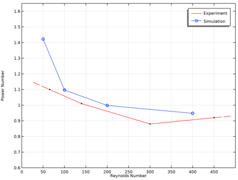
Click Replace Expression in the upper-right corner of the y-Axis Data section. From the menu, choose Component 1 (comp1)>Definitions>Variables>Np - Impeller power number.
5
Locate the x-Axis Data section. From the Parameter list, choose Expression.
6
Click Replace Expression in the upper-right corner of the x-Axis Data section. From the menu, choose Component 1 (comp1)>Definitions>Variables>NRe - Impeller Reynolds number.
7
Click to expand the Coloring and Style section. Find the Line markers subsection. From the Marker list, choose Circle.
8
From the Positioning list, choose In data points.
9
Click to expand the Legends section. From the Legends list, choose Manual.
10
Function 1
1
In the Model Builder window, click Function 1.
2
In the Settings window for Function, click to expand the Coloring and Style section.
3
From the Color list, choose Red.
4
Click to expand the Legends section. Select the Show legends check box.
5
From the Legends list, choose Manual.
6
Power number
1
In the Model Builder window, click Power number.
2
In the Settings window for 1D Plot Group, click to expand the Title section.
3
From the Title type list, choose None.
4
Locate the Plot Settings section. Select the x-axis label check box.
5
6
Select the y-axis label check box.
7
8
Locate the Axis section. Select the Manual axis limits check box.
9
In the x minimum text field, type 0.
10
In the x maximum text field, type 500.
11
In the y minimum text field, type 0.6.
12
In the y maximum text field, type 1.65.
13
In the Power number toolbar, click  Plot.
The following steps will reproduce Figure 3.
Cut Plane 1
1
In the Results toolbar, click  Cut Plane.
2
In the Settings window for Cut Plane, click  Plot.
Slice
1
In the Model Builder window, expand the Results>Velocity (spf) node, then click Slice.
2
In the Settings window for Slice, locate the Plane Data section.
3
From the Entry method list, choose Coordinates.
Arrow Surface 1
1
In the Model Builder window, right-click Velocity (spf) and choose Arrow Surface.
2
In the Settings window for Arrow Surface, locate the Data section.
3
From the Dataset list, choose Cut Plane 1.
4
Locate the Coloring and Style section. Select the Scale factor check box.
5
6
Locate the Arrow Positioning section. In the Number of arrows text field, type 500.
Surface 1
1
Right-click Velocity (spf) and choose Surface.
2
In the Settings window for Surface, locate the Data section.
3
From the Dataset list, choose All Walls.
4
Locate the Expression section. In the Expression text field, type 1.
5
Locate the Coloring and Style section. From the Coloring list, choose Uniform.
6
From the Color list, choose Gray.
Velocity (spf)
1
In the Model Builder window, click Velocity (spf).
2
In the Settings window for 3D Plot Group, locate the Plot Settings section.
3
Clear the Plot dataset edges check box.
4
Click to expand the Title section. From the Title type list, choose None.
5
Click the  Zoom Extents button in the Graphics toolbar.
Reproduce Figure 4 by the following steps.
Viscosity
1
Right-click Velocity (spf) and choose Duplicate.
2
Right-click Velocity (spf) 1 and choose Rename.
3
In the Rename 3D Plot Group dialog box, type Viscosity in the New label text field.
4
Slice
1
In the Model Builder window, expand the Viscosity node, then click Slice.
2
In the Settings window for Slice, locate the Expression section.
3
In the Expression text field, type log(spf.mu_app).
4
In the Viscosity toolbar, click  Plot.