|
|
|


|
|
|||
|
1
|
|
2
|
|
3
|
Click Add.
|
|
4
|
Click
|
|
5
|
|
6
|
Click
|
|
1
|
|
2
|
|
3
|
|
4
|
|
1
|
|
2
|
|
3
|
|
4
|
|
5
|
|
1
|
|
2
|
|
3
|
|
4
|
|
5
|
|
1
|
|
2
|
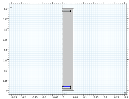
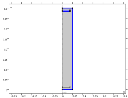
Select the object r1 only.
|
|
3
|
|
4
|
|
1
|
|
2
|
|
3
|
|
4
|
|
5
|
|
6
|
|
7
|
|
8
|
|
1
|
|
2
|
|
3
|
|
1
|
|
2
|
|
1
|
|
2
|
|
3
|
|
4
|
Click OK.
|
|
5
|
|
6
|
|
1
|
|
2
|
|
3
|
|
4
|
Click OK.
|
|
5
|
|
6
|
|
1
|
|
2
|
|
3
|
|
4
|
Click OK.
|
|
5
|
|
6
|
|
1
|
|
2
|
|
3
|
|
4
|
Click OK.
|
|
5
|
|
6
|
|
1
|
|
2
|
|
3
|
|
4
|
Click OK.
|
|
5
|
|
6
|
|
1
|
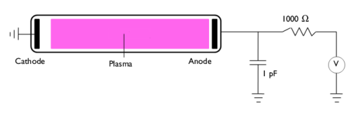
In the Model Builder window, under Component 1 (comp1) right-click Plasma (plas) and choose Global>Cross Section Import.
|
|
2
|
|
3
|
Click
|
|
5
|
Click
|
|
6
|
|
7
|
|
8
|
|
1
|
|
2
|
|
3
|
|
4
|
|
1
|
|
2
|
|
3
|
|
4
|
Locate the Reaction Parameters section. From the Rate constant form list, choose Townsend coefficient.
|
|
5
|
|
1
|
|
2
|
|
3
|
|
4
|
Locate the Reaction Parameters section. From the Rate constant form list, choose Townsend coefficient.
|
|
5
|
|
1
|
|
2
|
|
3
|
|
4
|
|
1
|
|
2
|
|
3
|
|
4
|
|
1
|
|
2
|
|
3
|
|
4
|
|
1
|
|
2
|
|
3
|
|
1
|
|
2
|
|
3
|
|
4
|
|
1
|
|
2
|
|
3
|
|
1
|
|
2
|
|
3
|
|
1
|
|
2
|
|
3
|
|
4
|
|
5
|
|
1
|
|
2
|
|
3
|
|
1
|
|
2
|
|
3
|
|
4
|
|
5
|
|
6
|
|
1
|
|
2
|
|
3
|
|
4
|
|
1
|
|
2
|
|
3
|
|
4
|
|
1
|
|
1
|
|
2
|
|
3
|
|
4
|
Click the Custom button.
|
|
5
|
|
6
|
|
7
|
|
1
|
|
2
|
|
3
|
|
1
|
|
2
|
|
3
|
|
4
|
|
5
|
|
1
|
|
2
|
|
3
|
|
4
|
Click
|
|
5
|
|
6
|
|
7
|
|
8
|
|
9
|
|
10
|
Click Add.
|
|
11
|
|
1
|
|
2
|
|
3
|
|
4
|
|
1
|
|
2
|
|
3
|
|
4
|
|
1
|
|
2
|
|
3
|
|
4
|
|
5
|
|
1
|
|
2
|
|
3
|
|
4
|
|
5
|
|
1
|
|
2
|
|
3
|
|
4
|
|
5
|
|
1
|
|
2
|
|
3
|
|
4
|
|
5
|
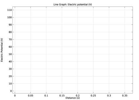
In the associated text field, type Distance (x).
|
|
6
|
|
7
|
In the associated text field, type Electric Potential (V).
|
|
8
|
|
1
|
|
2
|
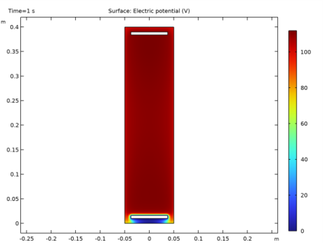
In the Settings window for Line Graph, click Replace Expression in the upper-right corner of the y-Axis Data section. From the menu, choose Component 1 (comp1)>Plasma>Electric>V - Electric potential - V.
|
|
1
|
|
2
|
|
3
|
|
1
|
|
2
|
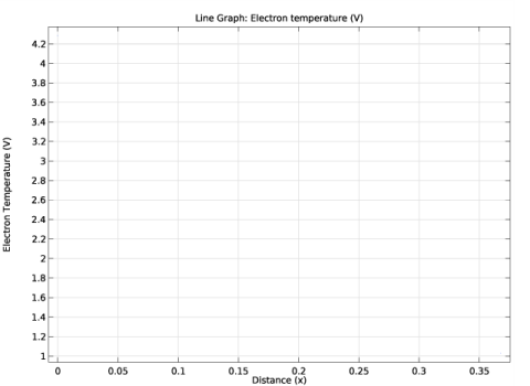
In the Settings window for 1D Plot Group, type Electron Temperature on Axis in the Label text field.
|
|
3
|
|
4
|
|
5
|
In the associated text field, type Distance (x).
|
|
6
|
|
7
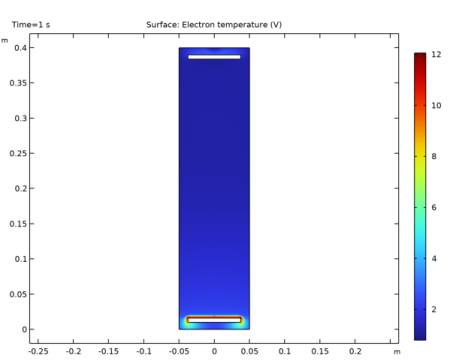
|
In the associated text field, type Electron Temperature (V).
|
|
8
|
|
1
|
|
2
|
|
3
|
|
4
|
|
5
|
|
1
|
|
2
|
|
3
|
|
4
|
|
5
|
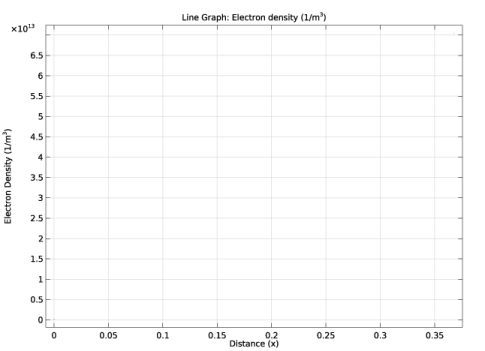
In the associated text field, type Distance (x).
|
|
6
|
|
7
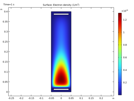
|
In the associated text field, type Electron Density (1/m<sup>3</sup>).
|
|
8
|
|
1
|
|
2
|
|
3
|
|
4
|
|
5
|
|
1
|
|
2
|
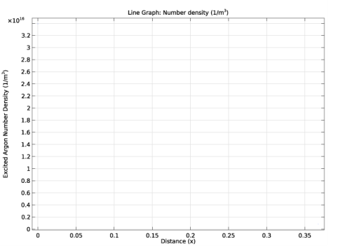
In the Settings window for 1D Plot Group, type Excited Argon Number Density on Axis in the Label text field.
|
|
3
|
|
4
|
|
5
|
In the associated text field, type Distance (x).
|
|
6
|
|
7
|
In the associated text field, type Excited Argon Number Density (1/m<sup>3</sup>).
|
|
8
|
|
1
|
|
2
|
|
3
|
|
4
|
|
5
|
|
1
|
|
2
|
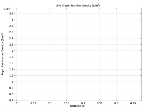
In the Settings window for 1D Plot Group, type Argon Ion Number Density on Axis in the Label text field.
|
|
3
|
|
4
|
|
5
|
In the associated text field, type Distance (x).
|
|
6
|
|
7
|
In the associated text field, type Argon Ion Number Density (1/m<sup>3</sup>).
|
|
8
|
|
1
|
|
2
|
|
3
|
|
4
|
|
5
|