Argon Boltzmann Analysis

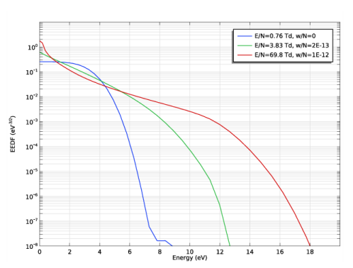
PDF

Argon Boltzmann Analysis

The electron energy distribution function (EEDF) plays an important role in the overall behavior of discharges. Analytic forms of the EEDF exist such as Maxwellian or Druyvesteyn, but in some cases they fail to fit the discharge physics. Factors such as ionization degree (ne/Nn), mole fraction of excited species, and reduced angular frequency of the electromagnetic field can all influence the shape of the EEDF. This can lead to differences in the magnitude of electron impact rate coefficients which are in turn used in a fluid model to solve for the electron density and mean electron energy. This tutorial model shows how these factors influence the EEDF and the rate coefficients for argon.

Model Definition

This tutorial is based on the results obtained in Ref. 1. The Two-term Boltzmann equation is solved which computes the EEDF rather than assuming a specific form. The Boltzmann equation in the two-term approximation can be written as

where f is the EEDF (eV−3/2) and

(1)

(2)

For definitions of the quantities in the equations Equation 1 and Equation 2, see the chapter The Boltzmann Equation, Two-Term Approximation Interface in the Plasma Module User’s Guide.

At zero energy, the condition that energy flux is zero must hold:

and as ε → ∞, f → 0.

The EEDF is defined by how electrons gain energy from the electric field and lose (or gain) their energy in collisions with the background gas. The electron collisions are characterized by cross sections that need to be provided by the user. In this model, the background gas is argon and the electron impact collisions listed in Table 1 below are considered (electron impact cross-sections are obtained from Ref. 2).

Table 1: Electron impact collisions.
reaction	Formula	Type	Δε (eV)
1	e+Ar=>e+Ar	Elastic	0
2	e+Ar=>e+Ars	Excitation	11.5
3	e+Ars=>e+Ar	Excitation	-11.5
4	e+Ar=>2e+Ar+	Ionization	15.8
5	e+Ars=>2e+Ar+	Ionization	4.4

Results and Discussion

In this section it is studied how the EEDF and the ionization rate coefficient are influenced by electron-electron collisions, superelastic collisions, and excitation frequency.

Electron-electron collisions tend to make the shape of the EEDF closer to a Maxwellian distribution function. The influence of these collisions depend mostly on the ionization degree. Figure 1 shows computed EEDFs for several ionization degrees for an electron density of 1018 m−3 and for a reduced electric field of 10 Td. As the ionization degree increases, the EEDF tends to become more Maxwellian (which would be represented by a linear line on a log scale).

The electron-electron collisions tend to push the electrons at the tail to higher energies, which has an effect on the rate coefficients for electron impact reactions with a high threshold energy. The effect on the ionization rate coefficient can be seen in Figure 2. In the low mean energy range the ionization rate coefficient increases considerable with the ionization degree.

Electrons can collide with neutrals in an excited state and cause them to de-excite to a low energy state. In this type of collisions the electrons can take the energy excess and immediately populate the tail of the EEDF. This effect on the EEDF is presented in Figure 3 for different mole fractions of the excited state of argon. The population of the high energy tail makes the magnitude of the ionization rate coefficients increase in the low energy range as shown in Figure 4.

Finally, the influence of a high frequency oscillating field on the EEDF and the ionization rate coefficients is studied by applying different excitation frequencies at a constant mean electron energy. The results are plotted in Figure 5 and Figure 6.

Figure 1: EEDF for 10 Td and for different ionization degrees.

Figure 2: Ionization rate coefficient as a function of the mean electron energy for different ionization degrees.

Figure 3: EEDF for 10 Td and for different mole fractions of the argon excited state.

Figure 4: Ionization rate coefficient as a function of the mean electron energy for different mole fractions of the argon excited state.

Figure 5: EEDF for oscillating electric fields with different amplitudes and different reduced frequencies. All EEDFs have the same mean electron energy of 2.15 eV.

Figure 6: Ionization rate coefficient as a function of the mean electron energy for different reduced frequencies.

1. G.J.M. Hagelaar and L.C. Pitchford, “Solving the Boltzmann Equation to Obtain Electron Transport Coefficients and Rate Coefficients for Fluid Models”, Plasma Sources Science and Technology, vol. 14, pp. 722–733, 2005.

2. Phelps database, www.lxcat.net, retrieved 2017.

Plasma_Module/Two-Term_Boltzmann_Equation/boltzmann_argon

Modeling Instructions

From the menu, choose .

In the window, click

.

1

In the window, Select the interface and the study.

2

3

In the tree, select .

4

5

6

In the tree, select .

7

Boltzmann Equation, Two-Term Approximation (be)

Select to solve the Boltzmann equation in the two-term approximation.

1

In the window, under click .

2

In the window for , locate the section.

3

From the list, choose .

4

Select the check box.

Define parameters for the ionization degree, Argon excited state mole fraction, and reduced oscillating frequency.

Global Definitions

1

In the window, under click .

2

In the window for , locate the section.

3

In the table, enter the following settings:


Name	Expression	Value	Description
Beta	0	0	Ionization degree
xArs	0	0	Ars mole fraction
wN	0	0	Reduced frequency

Import a cross section set for Argon.

Boltzmann Equation, Two-Term Approximation (be)

Cross Section Import 1

1

In the toolbar, click

and choose .

2

In the window for , locate the section.

3

4

Browse to the model’s Application Libraries folder and double-click the file Ar_xsecs.txt.

5

In the first two studies the effect of the electron-electron collisions on the eedf and the ionization rate coefficient are analyzed.

In the first study, compute the eedf for a constant reduced electric field for several ionization degrees.

In the second study, use the parametric sweep feature to compute the rate coefficients over a wide range of mean electron energies for different degrees of ionization.

Boltzmann Model 1

1

In the window, click .

2

In the window for , locate the section.

3

In the ne text field, type 1E18[1/m^3].

4

In the β text field, type Beta.

5

Locate the section. Find the subsection. Clear the check box.

6

Clear the check box.

7

Clear the check box.

Initial Values 1

1

In the window, click .

2

In the window for , locate the section.

3

In the ε0 text field, type 5[V].

4

In the E/N0 text field, type 10[Td].

1

In the window, click .

2

In the window for , type eedf e-e in the text field.

Step 1: Reduced Electric Fields

1

In the window, under click .

2

In the window for , locate the section.

3

In the text field, type 10[Td].

4

Click to expand the section. Select the check box.

5

6

In the table, enter the following settings:


Parameter name	Parameter value list	Parameter unit
Beta (Ionization degree)	0 1e-6 1e-5 1e-4 1e-3 1e-2

7

From the list, choose .

8

In the toolbar, click

.

1

In the window for , type EEDF e-e in the text field.

2

Locate the section. Select the check box.

3

In the text field, type 0.

4

In the text field, type 35.

5

In the text field, type 1e-9.

6

In the text field, type 1.

1

In the window, expand the node, then click .

2

In the window for , click to expand the section.

3

From the list, choose .

4

In the text field, type Beta = eval(Beta).

5

In the toolbar, click

.

1

In the toolbar, click

to open the window.

2

Go to the window.

3

Find the subsection. In the tree, select .

4

Click in the window toolbar.

5

In the toolbar, click

to close the window.

Step 1: Mean Energies

1

In the window for , locate the section.

2

3

In the dialog box, type 2 in the text field.

4

In the text field, type 0.2.

5

In the text field, type 10.

6

7

In the window, click .

8

In the window for , type Rion e-e in the text field.

9

Locate the section. Clear the check box.

10

Clear the check box.

Parametric Sweep

1

In the toolbar, click

.

2

In the window for , locate the section.

3

4

In the table, enter the following settings:


Parameter name	Parameter value list	Parameter unit
Beta (Ionization degree)	0 1e-6 1e-5 1e-4 1e-3 1e-2

5

In the toolbar, click

.

Ionization vs. electron mean energy e-e

1

In the toolbar, click

and choose .

2

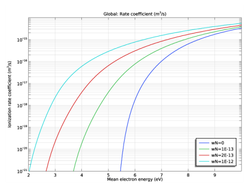
In the window for , type Ionization vs. electron mean energy e-e in the text field.

3

Locate the section. From the list, choose .

4

Locate the section. Select the check box.

5

In the associated text field, type Mean electron energy (eV).

6

Select the check box.

7

In the associated text field, type Ionization rate coefficient (m<sup>3</sup>/s).

8

Locate the section. Select the check box.

9

In the text field, type 2.

10

In the text field, type 10.

11

In the text field, type 1e-21.

12

In the text field, type 1e-14.

13

Select the check box.

14

Locate the section. From the list, choose .

1

Right-click and choose .

2

In the window for , locate the section.

3

In the table, enter the following settings:


Expression	Unit	Description
be.k_4	m^3/s	Rate coefficient

4

Click to expand the section. From the list, choose .

5

Find the subsection. Clear the check box.

6

In the toolbar, click

.

In the following, the effects of the Ars state mole fraction in the eedf are studied. Do not include electron-electron collisions and set the model fraction of xArs.

Boltzmann Equation, Two-Term Approximation (be)

1

In the window, under click .

2

In the window for , locate the section.

3

Clear the check box.

Boltzmann Model 1

1

In the window, under click .

2

In the window for , locate the section.

3

From the list, choose .

4

In the table, enter the following settings:


Species	Mole fraction (1)
Ars	xArs

As before two studies are made. The first study, parameterizes over the Ars mole fraction and serves to analyze the effects of superelastic reactions on the eedf.

The second study, parameterizes over the Ars mole fraction over a wide range of mean electron energies and serves to analyze the effects of superelastic reactions on the ionization rate coefficient.

1

In the toolbar, click

to open the window.

2

Go to the window.

3

Find the subsection. In the tree, select .

4

Click in the window toolbar.

5

In the toolbar, click

to close the window.

Step 1: Reduced Electric Fields

1

In the window for , locate the section.

2

In the text field, type 10[Td].

3

From the list, choose .

4

Locate the section. Select the check box.

5

6

In the table, enter the following settings:


Parameter name	Parameter value list	Parameter unit
xArs (Ars mole fraction)	0 1e-5 1e-4 1e-3

7

In the window, click .

8

In the window for , locate the section.

9

Clear the check box.

10

Clear the check box.

11

In the text field, type eedf xArs.

12

In the toolbar, click

.

1

In the window, right-click and choose .

2

In the window for , type EEDF xArs in the text field.

3

Locate the section. From the list, choose .

1

In the window, expand the node, then click .

2

In the window for , locate the section.

3

From the list, choose .

4

In the text field, type xArs= eval(xArs).

5

In the toolbar, click

.

1

In the toolbar, click

to open the window.

2

Go to the window.

3

Find the subsection. In the tree, select .

4

Click in the window toolbar.

5

In the toolbar, click

to close the window.

Step 1: Mean Energies

1

In the window for , locate the section.

2

3

In the dialog box, type 2 in the text field.

4

In the text field, type 0.2.

5

In the text field, type 10.

6

7

In the window, click .

8

In the window for , type Rion xArs in the text field.

9

Locate the section. Clear the check box.

10

Clear the check box.

Parametric Sweep

1

In the toolbar, click

.

2

In the window for , locate the section.

3

4

In the table, enter the following settings:


Parameter name	Parameter value list	Parameter unit
xArs (Ars mole fraction)	0 1e-5 1e-4 1e-3

5

In the toolbar, click

.

Ionization vs. electron mean energy xArs

1

In the window, right-click and choose .

2

In the window for , type Ionization vs. electron mean energy xArs in the text field.

3

Locate the section. From the list, choose .

1

In the window, expand the node, then click .

2

In the window for , locate the section.

3

From the list, choose .

4

Find the subsection. Clear the check box.

5

In the toolbar, click

.

Boltzmann Equation, Two-Term Approximation (be)

1

In the window, under click .

2

In the window for , locate the section.

3

Select the check box.

4

In the ω/N text field, type wN.

1

In the toolbar, click

to open the window.

2

Go to the window.

3

Find the subsection. In the tree, select .

4

Click in the window toolbar.

5

In the toolbar, click

to close the window.

Step 1: Reduced Electric Fields

In the following 3 EEDFs, all with the same mean electron energy of 2.15 eV, are computed for different reduced fields and reduced oscillating frequencies.

1

In the window for , locate the section.

2

In the text field, type 0.76[Td].

3

In the window, click .

4

In the window for , type 0.76Td w/N=0 in the text field.

5

Locate the section. Clear the check box.

6

Clear the check box.

7

In the toolbar, click

.

1

In the toolbar, click

to open the window.

2

Go to the window.

3

Find the subsection. In the tree, select .

4

Click in the window toolbar.

5

In the toolbar, click

to close the window.

Step 1: Reduced Electric Fields

1

In the window for , locate the section.

2

In the text field, type 3.83[Td].

3

Locate the section. Select the check box.

4

5

In the table, enter the following settings:


Parameter name	Parameter value list	Parameter unit
wN (Reduced frequency)	2e-13

6

In the window, click .

7

In the window for , type 3.83Td w/N=2e-13 in the text field.

8

Locate the section. Clear the check box.

9

Clear the check box.

10

In the toolbar, click

.

1

In the toolbar, click

to open the window.

2

Go to the window.

3

Find the subsection. In the tree, select .

4

Click in the window toolbar.

5

In the toolbar, click

to close the window.

Step 1: Reduced Electric Fields

1

In the window for , locate the section.

2

In the text field, type 69.8[Td].

3

Locate the section. Select the check box.

4

5

In the table, enter the following settings:


Parameter name	Parameter value list	Parameter unit
wN (Reduced frequency)	1e-12

6

In the window, click .

7

In the window for , type 69.8Td w/N=1e-12 in the text field.

8

Locate the section. Clear the check box.

9

Clear the check box.

10

In the toolbar, click

.

1

In the window, right-click and choose .

2

In the window for , locate the section.

3

From the list, choose .

4

Locate the section. In the text field, type 20.

5

In the text field, type 1e-8.

6

In the text field, type 10.

7

In the text field, type EEDF w/N.

1

In the window, expand the node, then click .

2

In the window for , locate the section.

3

From the list, choose .

4

In the text field, type E/N=eval(be.EN,Td,3) Td, w/N=eval(wN).

5

In the toolbar, click

.

1

Right-click and choose .

2

In the window for , locate the section.

3

From the list, choose .

1

Right-click and choose .

2

In the window for , locate the section.

3

From the list, choose .

4

In the toolbar, click

.

The last study parameterizes over the reduced oscillating frequency over a wide range of reduced electric fields.

1

In the toolbar, click

to open the window.

2

Go to the window.

3

Find the subsection. In the tree, select .

4

Click in the window toolbar.

5

In the toolbar, click

to close the window.

Step 1: Reduced Electric Fields

1

In the window for , locate the section.

2

3

In the dialog box, type 10 in the text field.

4

In the text field, type 5.

5

In the text field, type 2500.

6

7

In the window for , locate the section.

8

In the text field, type range(10,2,2500)[Td].

9

From the list, choose .

10

In the window, click .

11

In the window for , type Rion w/N in the text field.

12

Locate the section. Clear the check box.

13

Clear the check box.

Parametric Sweep

1

In the toolbar, click

.

2

In the window for , locate the section.

3

4

In the table, enter the following settings:


Parameter name	Parameter value list	Parameter unit
wN (Reduced frequency)	0 1e-13 2e-13 1e-12

5

In the toolbar, click

.

Ionization vs. electron mean energy w/N

1

In the window, right-click and choose .

2

In the window for , type Ionization vs. electron mean energy w/N in the text field.

3

Locate the section. From the list, choose .

1

In the window, expand the node, then click .

2

In the window for , locate the section.

3

From the list, choose .

4

In the text field, type be.ebar.

5

Locate the section. From the list, choose .

6

Find the subsection. Clear the check box.

7

In the toolbar, click

.