PDF

Stress in Cooling Pipeline Network
Introduction
This example demonstrates how to model coupled flow, heat transfer, and structural deformation in a pipe network. Gravity loads from the pipe and fluid are also taken into account.
Model Definition
The cooling system consists of a pipeline network spread over the floor as shown in Figure 1. The cooling fluid is water, and the flow is driven by a pump located at the ground flow. The heat is supplied to the inner spiral part of the pipeline, while the part of the pipeline located at the upper floor is cooled by the natural convection in the surrounding air. All other pipes are thermally insulated.
Figure 1: Geometry.
Model the pipeline in 3D as a system of connected edges using dedicated physics interfaces for computing pipe flow, pipe deformation, and heat transfer. The interfaces are based on the assumption that the diameter to length ratio is small enough to represent each individual pipe section as a 1D object. The simplified geometry is shown in Figure 2. The pump is replaced by a straight pipe section connecting the pump intake and outlet positions, making the pipe system closed. The pressure increase is specified at the point representing the pipe outlet, and the pressure is set to a reference value of 1 atm at the point representing the pipe intake.
Figure 2: Simplified model geometry. The blue and red colors represent the parts of the pipeline with the pipe inner diameter of 10 cm and 20 cm, respectively. The pump position and the flow direction is highlighted in green. The reference pressure of 1 atm is prescribed at the point highlighted in yellow.
A heat source of 300 W/m is applied at the spiral part of the pipeline, while its upper part is cooled by the natural convection in the surrounding air, which has the environment temperature of 20°C.
The pipes are made of structural steel with a wall thickness of 3 mm. The whole system is subjected to gravity. The pipes are mechanically constrained by various unidirectional supports located at certain points. The fluid overpressure and other flow-induced forces act on the pipe walls. In addition, the temperature increase and variation cause thermal expansion and stress in the pipeline sections.
Results and Discussion
Compute the flow, temperature distribution, and pipe deformation and stress for the pressure increase at the pump, dp, that gradually varies from 2 atm down to 0.25 atm. The resulting maximum temperature and maximum von Mises stress over the pipeline are shown in Figure 3 and Figure 4, respectively.
Figure 3: Maximum temperature.
Figure 4: Maximum von Mises stress.
The plots show that both quantities assume their lowest value at dp around 0.5 atm. Figure 5 shows the temperature distribution over the pipeline for that value of the parameter. Thus, the temperature increase is almost 30°C above the environment temperature. The performance can be considered acceptable since the total rate of removed heat is about 26 kW.
Figure 5: Temperature distribution for the pressure increase of 0.5 atm at the pump.
The fluid pressure and the velocity field for dp = 0.5 atm are shown in Figure 6 and Figure 7, respectively.
Figure 6: Fluid pressure distribution for the pressure increase of 0.5 atm at the pump.
Figure 7: Flow velocity field for the pressure increase of 0.5 atm at the pump.
The stress distribution in the pipeline is shown in Figure 8. The maximum von Mises stress is about 100 MPa, which is far below the yield strengths of the material.
Figure 8: von Mises stress in the deformed pipeline for the pressure increase of 0.5 atm at the pump.
The following two plots show the section force and moment.
Figure 9: Total bending moment for the pressure increase of 0.5 atm at the pump.
Figure 10: Total shear force for the pressure increase of 0.5 atm at the pump.
Notes About the COMSOL Implementation
Start the model setup by adding a Fluid-Pipe Interaction, Fixed Geometry multiphysics interface. This will bring in two physics interfaces, Pipe Flow and Pipe Mechanics, together with a multiphysics coupling feature, Fluid-Pipe Interaction.
The interfaces are unidirectionally coupled. Thus, the flow affects the structural displacement, but the pipeline geometry change because of the deformation is assumed to be small and will have no effect on the flow computations.
The flow-induced forces, such as internal overpressure, drag, and junction forces are computed and applied on the structure automatically by the coupling feature.
Later on in the modeling, you add a Heat Transfer in Pipes interface. This interface is based on the assumption that the main mechanism of the heat transfer along the pipe is heat convection due to the fluid flow. Thus, the heat conduction in the pipe walls in the direction along the pipe is neglected. Therefore, only the material representing the fluid is needed for the Heat Transfer in Pipes interface. The same applies to the Pipe Flow interface. Since both interfaces can take data from an active material with proper selection made under Materials in the component, add the fluid material (water in this case) as the last one to avoid overriding.
The Pipe Mechanics interface needs two materials, one for the pipe wall and the other for the contained fluid. The materials are chosen in the node Fluid and Pipe Materials under the interface. The material selection lists contain all materials available in the component. The material data are taken from the selected material even if the corresponding material node has no selection or is overridden under Materials in the component.
Application Library path: Pipe_Flow_Module/Pipe_Mechanics/cooling_pipeline_stress
Modeling Instructions
From the File menu, choose New.
New
In the New window, click  Model Wizard.
Model Wizard
1
In the Model Wizard window, click  3D.
2
In the Select Physics tree, select Structural Mechanics>Fluid-Structure Interaction>Fluid-Pipe Interaction, Fixed Geometry.
3
Click Add.
4
Click  Study.
5
In the Select Study tree, select General Studies>Stationary.
6
Global Definitions
Parameters 1
1
In the Model Builder window, under Global Definitions click Parameters 1.
2
In the Settings window for Parameters, locate the Parameters section.
3
Build the geometry using predefined polygons representing different parts of the pipeline.
Geometry 1
Polygon 1 (pol1)
1
In the Geometry toolbar, click  More Primitives and choose Polygon.
2
In the Settings window for Polygon, locate the Coordinates section.
3
Click  Load from File.
4
5
Locate the Selections of Resulting Entities section. Select the Resulting objects selection check box.
6
Find the Cumulative selection subsection. Click New.
7
In the New Cumulative Selection dialog box, type piping_main in the Name text field.
8
Polygon 2 (pol2)
1
In the Geometry toolbar, click  More Primitives and choose Polygon.
2
In the Settings window for Polygon, locate the Coordinates section.
3
Click  Load from File.
4
5
Locate the Selections of Resulting Entities section. Select the Resulting objects selection check box.
6
Find the Cumulative selection subsection. Click New.
7
In the New Cumulative Selection dialog box, type piping_inlet in the Name text field.
8
Polygon 3 (pol3)
1
In the Geometry toolbar, click  More Primitives and choose Polygon.
2
In the Settings window for Polygon, locate the Coordinates section.
3
Click  Load from File.
4
5
Locate the Selections of Resulting Entities section. Select the Resulting objects selection check box.
6
Find the Cumulative selection subsection. Click New.
7
In the New Cumulative Selection dialog box, type piping_outlet in the Name text field.
8
Polygon 4 (pol4)
1
In the Geometry toolbar, click  More Primitives and choose Polygon.
2
In the Settings window for Polygon, locate the Coordinates section.
3
Click  Load from File.
4
5
Locate the Selections of Resulting Entities section. Select the Resulting objects selection check box.
6
Find the Cumulative selection subsection. Click New.
7
In the New Cumulative Selection dialog box, type piping_heater in the Name text field.
8
Partition certain edges to add points where the pipeline will be mechanically supported.
Partition Edges 1 (pare1)
1
In the Geometry toolbar, click  Booleans and Partitions and choose Partition Edges.
2
In the Settings window for Partition Edges, locate the Edge Selection section.
3
Click  Paste Selection.
4
In the Paste Selection dialog box, type pol1: 1-3, 6, 32, 33 in the Selection text field.
5
6
In the Settings window for Partition Edges, locate the Positions section.
7
Partition Edges 2 (pare2)
1
In the Geometry toolbar, click  Booleans and Partitions and choose Partition Edges.
2
In the Settings window for Partition Edges, locate the Edge Selection section.
3
Click  Paste Selection.
4
In the Paste Selection dialog box, type pare1: 7, 8, 11, 20 pol3: 3 in the Selection text field.
5
6
In the Settings window for Partition Edges, locate the Positions section.
7
Partition Edges 3 (pare3)
1
In the Geometry toolbar, click  Booleans and Partitions and choose Partition Edges.
2
In the Settings window for Partition Edges, locate the Edge Selection section.
3
Click  Paste Selection.
4
In the Paste Selection dialog box, type pare2(1): 12, 16, 23, 29 pol2: 3, 4 pol4: 3 in the Selection text field.
5
Define a work plane and the corresponding boundary coordinate system to be used in the support definition.
Work Plane 1 (wp1)
1
In the Geometry toolbar, click  Work Plane.
2
In the Settings window for Work Plane, locate the Plane Definition section.
3
From the Plane type list, choose Vertices.
4
Click the  Zoom Box button in the Graphics toolbar.
5
On the object pare3(3), select Point 2 only.
6
Find the Second vertex subsection. Click to select the  Activate Selection toggle button.
7
On the object pare3(3), select Point 25 only.
8
Find the Third vertex subsection. Click to select the  Activate Selection toggle button.
9
On the object pare3(3), select Point 1 only.
10
Click  Build All Objects.
Definitions
System from Geometry 2 (sys2)
1
In the Definitions toolbar, click  Coordinate Systems and choose System from Geometry.
2
In the Settings window for System from Geometry, locate the System from Geometry section.
3
From the Work plane list, choose Work Plane 1 (wp1).
Define variables for the pipe inner diameter for different parts of the pipeline.
Variables 1
1
In the Model Builder window, right-click Definitions and choose Variables.
2
In the Settings window for Variables, locate the Variables section.
3
4
Locate the Geometric Entity Selection section. From the Geometric entity level list, choose Edge.
5
From the Selection list, choose piping_main.
Variables 2
1
Right-click Variables 1 and choose Duplicate.
2
In the Settings window for Variables, locate the Geometric Entity Selection section.
3
From the Selection list, choose piping_heater.
Variables 3
1
Right-click Variables 2 and choose Duplicate.
2
In the Settings window for Variables, locate the Variables section.
3
4
Locate the Geometric Entity Selection section. From the Selection list, choose piping_inlet.
Variables 4
1
Right-click Variables 3 and choose Duplicate.
2
In the Settings window for Variables, locate the Geometric Entity Selection section.
3
From the Selection list, choose piping_outlet.
Define a maximum operator to be used in the result analysis.
Maximum 1 (maxop1)
1
In the Definitions toolbar, click  Nonlocal Couplings and choose Maximum.
2
In the Settings window for Maximum, locate the Source Selection section.
3
From the Geometric entity level list, choose Edge.
4
From the Selection list, choose All edges.
The pipe walls are made of structural steel, the fluid inside is water, and the surrounding medium is air. The latter is needed for the specification of the cooling section of the pipeline.
Add Material
1
In the Home toolbar, click  Add Material to open the Add Material window.
2
Go to the Add Material window.
3
In the tree, select Built-in>Structural steel.
4
Right-click and choose Add to Component 1 (comp1).
5
6
Right-click and choose Add to Component 1 (comp1).
Materials
Air (mat2)
1
In the Model Builder window, under Component 1 (comp1)>Materials click Air (mat2).
2
In the Settings window for Material, locate the Geometric Entity Selection section.
3
From the Selection list, choose piping_main.
Add Material
1
Go to the Add Material window.
2
In the tree, select Built-in>Water, liquid.
3
Right-click and choose Add to Component 1 (comp1).
4
In the Home toolbar, click  Add Material to close the Add Material window.
Materials
Water, liquid (mat3)
1
In the Settings window for Material, locate the Geometric Entity Selection section.
2
From the Selection list, choose All edges.
Pipe Flow (pfl)
Fluid Properties 1
1
In the Model Builder window, under Component 1 (comp1)>Pipe Flow (pfl) click Fluid Properties 1.
2
In the Settings window for Fluid Properties, locate the Model Input section.
3
In the T text field, type 50[degC].
Pipe Properties 1
1
In the Model Builder window, click Pipe Properties 1.
2
In the Settings window for Pipe Properties, locate the Pipe Shape section.
3
4
In the di text field, type di.
5
Locate the Flow Resistance section. From the Surface roughness list, choose Commercial steel (0.046 mm).
Pipe Mechanics (pipem)
Fluid and Pipe Materials 1
1
In the Model Builder window, under Component 1 (comp1)>Pipe Mechanics (pipem) click Fluid and Pipe Materials 1.
2
In the Settings window for Fluid and Pipe Materials, locate the Pipe Properties section.
3
From the Pipe material list, choose Structural steel (mat1).
Pipe Cross Section 1
1
In the Model Builder window, click Pipe Cross Section 1.
2
In the Settings window for Pipe Cross Section, locate the Pipe Shape section.
3
4
In the di text field, type di.
5
In the do text field, type di+hpw.
Add the gravity force acting on the fluid. Note that the force defined here will only be accounted for when computing the flow in the pipeline.
Pipe Flow (pfl)
In the Model Builder window, under Component 1 (comp1) click Pipe Flow (pfl).
Volume Force 1
1
In the Physics toolbar, click  Edges and choose Volume Force.
2
In the Settings window for Volume Force, locate the Edge Selection section.
3
From the Selection list, choose All edges.
Add a pump node and define the pressure increase at its selected location.
Pump 1
1
In the Physics toolbar, click  Points and choose Pump.
2
3
In the Settings window for Pump, locate the Pump Specification section.
4
From the Type list, choose Pressure increase.
5
In the Δp text field, type dp.
Define the reference pressure.
Internal Pressure Lock 1
1
In the Physics toolbar, click  Points and choose Internal Pressure Lock.
2
Define two T-junctions in the pipeline.
T-junction 1
1
In the Physics toolbar, click  Points and choose T-junction.
2
In the Settings window for T-junction, locate the Selection Settings section.
3
Clear the Manual control of selections check box.
Bend 1
1
In the Physics toolbar, click  Points and choose Bend.
2
In the Settings window for Bend, locate the Point Selection section.
3
Click  Paste Selection.
4
In the Paste Selection dialog box, type 1-3, 7, 10-22, 25, 26, 28, 30, 32, 34-46, 48, 57, 59-61, 63-67, 69, 70, 77-80, 82-86, 90-96, 100, 101, 105 in the Selection text field.
5
This selection corresponds to all geometry turns except those used in the setup of the three previous nodes.
Initial Values 1
1
In the Model Builder window, click Initial Values 1.
2
In the Settings window for Initial Values, locate the Initial Values section.
3
In the ufluid text field, type -1.
Next, add the gravity force acting on the pipeline. The weights of both the pipe walls and the containing fluid will be taken into account in the force computations.
Pipe Mechanics (pipem)
In the Model Builder window, under Component 1 (comp1) click Pipe Mechanics (pipem).
Gravity 1
1
In the Physics toolbar, click  Edges and choose Gravity.
2
In the Settings window for Gravity, locate the Edge Selection section.
3
From the Selection list, choose All edges.
Fixed Constraint 1
1
In the Physics toolbar, click  Points and choose Fixed Constraint.
2
Define other mechanical constraints applied to the pipeline by using unidirectional supports.
Prescribed Displacement/Rotation 1
1
In the Physics toolbar, click  Points and choose Prescribed Displacement/Rotation.
2
In the Settings window for Prescribed Displacement/Rotation, locate the Point Selection section.
3
Click  Paste Selection.
4
In the Paste Selection dialog box, type 2-7, 10, 12, 14, 16, 18, 20, 22-34, 36, 38, 40, 42, 44, 46-49, 51-60, 63-65, 67, 68, 70-84, 86-105 in the Selection text field.
5
At these locations, the pipeline is supported, which will constrain its downward motion.
6
In the Settings window for Prescribed Displacement/Rotation, locate the Prescribed Displacement section.
7
From the Prescribed in z direction list, choose Limited.
8
In the u0z,min text field, type 0.
Prescribed Displacement/Rotation 2
1
In the Physics toolbar, click  Points and choose Prescribed Displacement/Rotation.
2
In the Settings window for Prescribed Displacement/Rotation, locate the Point Selection section.
3
Click  Paste Selection.
4
In the Paste Selection dialog box, type 62 in the Selection text field.
5
Here, possible horizontal motion of the T-junction will be restricted.
6
In the Settings window for Prescribed Displacement/Rotation, locate the Prescribed Displacement section.
7
From the Prescribed in x direction list, choose Limited.
8
In the u0x,max text field, type 0.01.
Prescribed Displacement/Rotation 3
1
In the Physics toolbar, click  Points and choose Prescribed Displacement/Rotation.
2
In the Settings window for Prescribed Displacement/Rotation, locate the Point Selection section.
3
Click  Paste Selection.
4
In the Paste Selection dialog box, type 50 in the Selection text field.
5
At this location, possible swaying of the pipe will be restricted.
6
In the Settings window for Prescribed Displacement/Rotation, locate the Coordinate System Selection section.
7
From the Coordinate system list, choose System from Geometry 2 (sys2).
8
Locate the Prescribed Displacement section. From the Prescribed in x2 direction list, choose Limited.
9
In the u0x2,max text field, type 0.
10
From the Prescribed in x3 direction list, choose Limited.
11
In the u0x3,max text field, type 0.01.
12
In the u0x3,min text field, type -0.01.
Before adding a Heat Transfer interface, generate a solver sequence. The Pipe Flow and Pipe Mechanics interfaces added so far to the model are unidirectionally coupled. Thus, the flow will affect the structural displacement, but not vice versa. The autogenerated solver sequence will use a segregated solver with two groups, where the fluid flow and structural displacement are computed consecutively.
Study 1
Solution 1 (sol1)
In the Study toolbar, click  Show Default Solver.
Add Physics
1
In the Home toolbar, click  Add Physics to open the Add Physics window.
2
Go to the Add Physics window.
3
In the tree, select Heat Transfer>Heat Transfer in Pipes (htp).
4
Click Add to Component 1 in the window toolbar.
5
In the Home toolbar, click  Add Physics to close the Add Physics window.
Heat Transfer in Pipes (htp)
Heat Transfer 1
1
In the Model Builder window, under Component 1 (comp1)>Heat Transfer in Pipes (htp) click Heat Transfer 1.
2
In the Settings window for Heat Transfer, locate the Heat Convection and Conduction section.
3
From the u list, choose Tangential velocity (pfl).
Pipe Properties 1
1
In the Model Builder window, click Pipe Properties 1.
2
In the Settings window for Pipe Properties, locate the Pipe Shape section.
3
4
In the di text field, type di.
5
Locate the Flow Resistance section. From the Surface roughness list, choose Commercial steel (0.046 mm).
Heat Source 1
1
In the Physics toolbar, click  Edges and choose Heat Source.
Specify the heat source location and intensity.
2
In the Settings window for Heat Source, locate the Edge Selection section.
3
Click  Paste Selection.
4
In the Paste Selection dialog box, type 12, 13, 15-29, 44-49 in the Selection text field.
5
This selection corresponds to the inner spiral part of the geometry.
6
In the Settings window for Heat Source, locate the Heat Source section.
7
In the Q text field, type Q.
Wall Heat Transfer 1
1
In the Physics toolbar, click  Edges and choose Wall Heat Transfer.
Define the top part of the pipeline, which is cooled by the surrounding air.
2
In the Settings window for Wall Heat Transfer, locate the Edge Selection section.
3
Click  Paste Selection.
4
In the Paste Selection dialog box, type 4-9, 30-34, 39-43, 51-54, 56, 59-64, 69, 73, 76-87, 90-106 in the Selection text field.
5
This selection corresponds to the top part of the geometry.
6
In the Settings window for Wall Heat Transfer, locate the Heat Transfer Model section.
7
In the Text text field, type Text.
Internal Film Resistance 1
In the Physics toolbar, click  Attributes and choose Internal Film Resistance.
Wall Heat Transfer 1
In the Model Builder window, click Wall Heat Transfer 1.
External Film Resistance 1
1
In the Physics toolbar, click  Attributes and choose External Film Resistance.
2
In the Settings window for External Film Resistance, locate the Specification section.
3
From the External film heat transfer model list, choose External natural convection.
4
From the Surrounding fluid list, choose Air (mat2).
Specify the thermal expansion of the pipe walls caused by the temperature increase and variation.
Pipe Mechanics (pipem)
Fluid and Pipe Materials 1
In the Model Builder window, under Component 1 (comp1)>Pipe Mechanics (pipem) click Fluid and Pipe Materials 1.
Thermal Expansion 1
1
In the Physics toolbar, click  Attributes and choose Thermal Expansion.
2
In the Settings window for Thermal Expansion, locate the Model Input section.
3
From the T list, choose Temperature (htp).
4
From the Tref list, choose User defined. In the associated text field, type Text.
Update the dependent variables in the solver, which will create a new segregated group for the variables added by the Heat Transfer interface.
Study 1
Solution 1 (sol1)
1
In the Model Builder window, expand the Study 1>Solver Configurations>Solution 1 (sol1) node.
2
Right-click Study 1>Solver Configurations>Solution 1 (sol1)>Dependent Variables 1 and choose Update Variables.
3
In the Model Builder window, expand the Study 1>Solver Configurations>Solution 1 (sol1)>Stationary Solver 1 node.
Configure the solver settings for the new segregated group to be similar to those for the two other groups.
4
In the Model Builder window, expand the Study 1>Solver Configurations>Solution 1 (sol1)>Stationary Solver 1>Segregated 1 node, then click Segregated Step 1.
5
In the Settings window for Segregated Step, type Heat in the Label text field.
6
Click to expand the Method and Termination section. From the Nonlinear method list, choose Automatic (Newton).
7
In the Tolerance factor text field, type 1.
8
In the Maximum number of iterations text field, type 50.
Move the group up so that the heat-transfer problem is solved after the flow computation but before the structural-displacement calculation.
9
Right-click Study 1>Solver Configurations>Solution 1 (sol1)>Stationary Solver 1>Segregated 1>Heat and choose Move Up.
Prepare a plot to be shown during the parametric-sweep computation.
10
In the Study toolbar, click  Show Default Plots.
Results
Line 1
1
In the Model Builder window, expand the Results>Temperature (htp) node, then click Line 1.
2
In the Settings window for Line, locate the Expression section.
3
From the Unit list, choose degC.
4
Locate the Coloring and Style section. Select the Radius scale factor check box.
5
Study 1
Step 1: Stationary
1
In the Model Builder window, under Study 1 click Step 1: Stationary.
2
In the Settings window for Stationary, click to expand the Results While Solving section.
3
Select the Plot check box.
4
From the Plot group list, choose Temperature (htp).
The pressure increase at the pump will gradually decrease from 2 atm down to 0.25 atm.
5
Click to expand the Study Extensions section. Select the Auxiliary sweep check box.
6
7
8
In the Study toolbar, click  Compute.
Results
Pressure (pfl)
Plot the maximum values of the temperature and the von Mises stress reached along the pipeline for all computed values of the pressure increase.
Maximum temperature
1
In the Home toolbar, click  Add Plot Group and choose 1D Plot Group.
2
In the Settings window for 1D Plot Group, type Maximum temperature in the Label text field.
3
Locate the Legend section. Clear the Show legends check box.
Global 1
1
Right-click Maximum temperature and choose Global.
2
In the Settings window for Global, locate the y-Axis Data section.
3
4
In the Maximum temperature toolbar, click  Plot.
Maximum von Mises stres
1
In the Model Builder window, right-click Maximum temperature and choose Duplicate.
2
In the Settings window for 1D Plot Group, type Maximum von Mises stres in the Label text field.
Global 1
1
In the Model Builder window, expand the Maximum von Mises stres node, then click Global 1.
2
In the Settings window for Global, locate the y-Axis Data section.
3
4
In the Maximum von Mises stres toolbar, click  Plot.
The plots should be similar to those shown in Figure 3 and Figure 4. They show that both quantities reaches their local minimum value for the pressure increase of 0.5 atm.
Update the default plots to select this value of dp parameter.
Pressure (pfl)
1
In the Model Builder window, under Results click Pressure (pfl).
2
In the Settings window for 3D Plot Group, locate the Data section.
3
From the Parameter value (dp (atm)) list, choose 0.5.
Line 1
1
In the Model Builder window, expand the Pressure (pfl) node, then click Line 1.
2
In the Settings window for Line, locate the Expression section.
3
From the Unit list, choose atm.
4
Locate the Coloring and Style section. Select the Radius scale factor check box.
5
6
In the Pressure (pfl) toolbar, click  Plot.
Velocity (pfl)
1
In the Model Builder window, under Results click Velocity (pfl).
2
In the Settings window for 3D Plot Group, locate the Data section.
3
From the Parameter value (dp (atm)) list, choose 0.5.
Arrow Line 1
1
In the Model Builder window, expand the Velocity (pfl) node, then click Arrow Line 1.
2
In the Settings window for Arrow Line, locate the Arrow Positioning section.
3
In the Number of arrows text field, type 80.
4
Locate the Coloring and Style section. From the Arrow type list, choose Cone.
5
From the Arrow base list, choose Center.
6
Select the Scale factor check box.
7
8
In the Velocity (pfl) toolbar, click  Plot.
Stress (pipem)
1
In the Model Builder window, under Results click Stress (pipem).
2
In the Settings window for 3D Plot Group, locate the Data section.
3
From the Parameter value (dp (atm)) list, choose 0.5.
Line 1
1
In the Model Builder window, expand the Stress (pipem) node, then click Line 1.
2
In the Settings window for Line, locate the Expression section.
3
From the Unit list, choose MPa.
4
Locate the Coloring and Style section. In the Radius scale factor text field, type 3.
5
From the Color table list, choose Rainbow.
Deformation
1
In the Model Builder window, expand the Line 1 node, then click Deformation.
2
In the Settings window for Deformation, locate the Scale section.
3
Select the Scale factor check box.
4
5
In the Stress (pipem) toolbar, click  Plot.
Temperature (htp)
1
In the Model Builder window, under Results click Temperature (htp).
2
In the Settings window for 3D Plot Group, locate the Data section.
3
From the Parameter value (dp (atm)) list, choose 0.5.
4
In the Temperature (htp) toolbar, click  Plot.
Total Bending Moment (pipem)
1
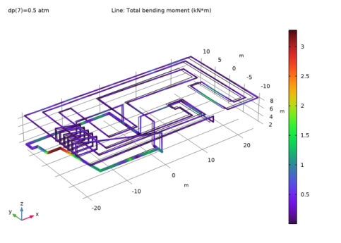
In the Model Builder window, expand the Results>Section Forces (pipem) node, then click Total Bending Moment (pipem).
2
In the Settings window for 3D Plot Group, locate the Data section.
3
From the Parameter value (dp (atm)) list, choose 0.5.
Line 1
1
In the Model Builder window, expand the Total Bending Moment (pipem) node, then click Line 1.
2
In the Settings window for Line, locate the Expression section.
3
From the Unit list, choose kN*m.
4
Locate the Coloring and Style section. In the Radius scale factor text field, type 3.
Deformation
1
In the Model Builder window, expand the Line 1 node, then click Deformation.
2
In the Settings window for Deformation, locate the Scale section.
3
Select the Scale factor check box.
4
5
In the Total Bending Moment (pipem) toolbar, click  Plot.
Total Shear Force (pipem)
1
In the Model Builder window, under Results>Section Forces (pipem) click Total Shear Force (pipem).
2
In the Settings window for 3D Plot Group, locate the Data section.
3
From the Parameter value (dp (atm)) list, choose 0.5.
Line 1
1
In the Model Builder window, expand the Total Shear Force (pipem) node, then click Line 1.
2
In the Settings window for Line, locate the Expression section.
3
From the Unit list, choose kN.
4
Locate the Coloring and Style section. In the Radius scale factor text field, type 3.
Deformation
1
In the Model Builder window, expand the Line 1 node, then click Deformation.
2
In the Settings window for Deformation, locate the Scale section.
3
Select the Scale factor check box.
4
5
In the Total Shear Force (pipem) toolbar, click  Plot.