Multistudy Optimization of a Bracket

In some application fields, there is a strong focus on weight reduction. For example, this is the case in the automotive industry, where every gram has a distinct price tag.

In this model, the weight of a mounting bracket is reduced, given an upper bound on the stresses and a lower bound on the first natural frequency.

The bracket is used for mounting a heavy component on a vibrating foundation. It is thus important to keep the natural frequency well above the excitation frequency in order to avoid resonances. The bracket is also subjected to shock loads, which can be treated as a static acceleration load. This gives an optimization problem, where results from two different study types must be considered simultaneously.

This application requires the Structural Mechanics Module and the Design Module.

Model Definition

The original bracket together with a sketched mounted component are shown in Figure 1. The bracket is made of steel.

The component, which can be considered as rigid when compared with the bracket, has its center of gravity at the center of the circular cutout in the bracket. The mass is 4.4 kg, the moment of inertia around its longitudinal axis is 7.1·10−4 kg·m2, and the moment of inertia around the two transverse axes is 9.3·10−4 kg·m2.

Figure 1: Bracket supporting a heavy component.

The idea is to reduce the weight by drilling holes in the vertical surface of the bracket, and at the same time change the dimensions of the indentations, in order to offset the loss in stiffness.

Optimization Parameters

Six geometrical parameters are used in the optimization. They are summarized in Table 1 and shown in Figure 2.

Table 1: Geometrical parameters.
Parameter	Description	Lower limit (mm)	Upper limit (mm)
rC	Radius of the central hole	3	15
zCo	Vertical distance from the bend to the edge of the central hole	1	23
rO	Radius of the outer hole	3	15
zOo	Vertical distance from the bend to the edge of the outer hole	8	30
yOo	Horizontal distance from the edge of the bracket to outer hole	3	29
wInd	Width of the indentation	8	20

Figure 2: Optimization parameters.

Constraints

•

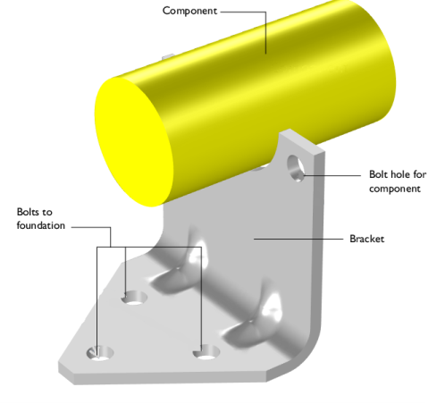
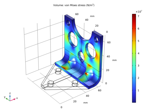
The lowest natural frequency must be at least 60 Hz.

•

When exposed to a peak acceleration of 4g in all three global directions simultaneously, the equivalent stress is not allowed to exceed 80 MPa anywhere. This criterion is nondifferentiable, because the location of the peak stress can jump from one place to another. A gradient-free optimization algorithm must thus be used.

•

There must be at least 3 mm of material between two holes, or between a hole and an edge. This criterion is enforced both through the limits on the control parameters and as constraints. The geometrical constraints are shown in Figure 3.

Figure 3: Geometrical constraints.

The COBYLA solver uses sampling in the control variable space to approximate both the objective function, the constraints, and the control variable bounds. Individual samples may be computed outside the bounds and in violation of the constraints. Therefore, it is important to parameterize the geometry in such a way that it is robust with respect to (small) constraint and bound violations.

Bounds and linear constraints are generally satisfied to high precision at the optimum point returned by the solver, but nonlinear constrains are often slightly violated. The reason is that the solver tends to converge from the outside of the feasible domain and terminates before the constraints are completely satisfied. Tightening the solver tolerances will decrease the constraint violation but is often not worth the computational effort; it is better to specify constraints with a safety margin.

Results and Discussion

The initial geometry used in the optimization is shown in Figure 4. Three rather small holes have been introduced.

Figure 4: Initial geometry.

The optimal values of the geometrical parameters are shown in Table 2.

Table 2: Optimal values.
Parameter	Optimal value (mm)	Lower limit (mm)	Upper limit (mm)
rC	11.8	3	15
zCo	2.7	1	23
rO	9.0	3	15
zOo	9.5	8	30
yOo	22.3	3	29
wInd	20	8	20

The weight of the optimized bracket is about 178 g, a reduction of 27 g from the original 205 g. The stresses from the shock load on the optimized geometry are shown in Figure 5

Figure 5: Stresses at peak load in the optimized design.

The optimal solution gives three fairly large holes, and the widest possible indentation.

There are several possible arrangements of the holes that give the same weight reduction within a small tolerance. It is therefore possible that the design variables are not always the same at convergence.

Notes About the COMSOL Implementation

The component mounted on the bracket is not modeled in detail. It is replaced by a Rigid Connector having the equivalent inertial properties.

Optimization_Module/Design_Optimization/multistudy_bracket_optimization

Modeling Instructions

From the menu, choose .

New

In the window, click

Model Wizard

In the window, click

In the tree, select .

Click .

Click

In the tree, select .

Click

Global Definitions

Parameters 1

In the window, under click .

In the window for , locate the section.

Click

Browse to the model’s Application Libraries folder and double-click the file multistudy_bracket_optimization_params.txt.

Geometry 1

In the window, under click .

In the window for , locate the section.

From the list, choose .

Locate the section. From the list, choose .

Select the check box.

The geometry sequence for the model (see Figure 1) is available in a file. If you want to create it from scratch yourself, you can follow the instructions in the Geometry Modeling Instructions section. Otherwise, insert the geometry sequence as follows:

In the toolbar, click

Browse to the model’s Application Libraries folder and double-click the file multistudy_bracket_optimization_geom_sequence.mph.

In the toolbar, click

Add Material

In the toolbar, click

to open the window.

Go to the window.

In the tree, select .

Click in the window toolbar.

In the toolbar, click

to close the window.

Solid Mechanics (solid)

Fixed (Bolts)

In the window, under right-click and choose .

The exact way the bolts clamp the bracket to the foundation is not important for the results in the part being optimized.

In the window for , type Fixed (Bolts) in the text field.

Select Boundaries 10–13 and 15–22 only.

Rigid Connector (Mounted component)

In the toolbar, click

and choose .

The attached component has a high stiffness, and is bolted to the two upper bolt holes. It is modeled as being rigid, with only mass properties.

In the window for , type Rigid Connector (Mounted component) in the text field.

Select Boundaries 48, 49, 52, 53, and 75–78 only.

Locate the section. From the list, choose .

Specify the Xc vector as


lX-thk/2	x
lY/2	y
lZ	z

Mass and Moment of Inertia 1

In the toolbar, click

and choose .

In the window for , locate the section.

In the m text field, type mCmp.

From the list, choose .

In the I table, enter the following settings:


IXCmp	0	0
0	IYZCmp	0
0	0	IYZCmp

Mesh 1

Free Triangular 1

In the toolbar, click

and choose .

Select Boundaries 4, 8, 26, 30, 35, 39, 41, 44, 60, and 64 only.

Size 1

Right-click and choose .

In the window for , locate the section.

From the list, choose .

Select Boundaries 4, 8, 26, 30, 44, and 64 only.

Size 2

Right-click and choose .

In the window for , locate the section.

From the list, choose .

Locate the section. Click

Select Boundaries 35, 39, 41, and 60 only.

Click

Swept 1

In the toolbar, click

Distribution 1

Right-click and choose .

In the window for , locate the section.

In the text field, type 3.

Click

Eigenfrequency Study

Run an eigenfrequency study on the initial geometry.

In the window, click .

In the window for , type Eigenfrequency Study in the text field.

In the toolbar, click

Solid Mechanics (solid)

Add the peak loads, and perform a stationary study.

Body load 4g on bracket

In the toolbar, click

and choose .

In the window for , type Body load 4g on bracket in the text field.

Locate the section. From the list, choose .

Locate the section. Specify the FV vector as


4g_constsolid.rho	x
4g_constsolid.rho	y
4g_constsolid.rho	z

Rigid Connector (Mounted component)

In the window, click .

Force 4g on mounted component

In the toolbar, click

and choose .

In the window for , type Force 4g on mounted component in the text field.

Locate the section. Specify the F vector as


4g_constmCmp	x
4g_constmCmp	y
4g_constmCmp	z

Add Study

In the toolbar, click

to open the window.

Go to the window.

Find the subsection. In the tree, select .

Click in the window toolbar.

In the toolbar, click

to close the window.

Stationary Study

In the window, click .

In the window for , type Stationary Study in the text field.

In the toolbar, click

Definitions

Prepare for the optimization by adding variables for the bracket mass and the maximum stress.

Domain Probe 1 (dom1)

In the toolbar, click

and choose .

In the window for , type mass in the text field.

Locate the section. From the list, choose .

Click in the upper-right corner of the section. From the menu, choose .

Boundary Probe 1 (bnd1)

In the toolbar, click

and choose .

In the window for , type maxStress in the text field.

Locate the section. From the list, choose .

Select Boundaries 25, 26, 29, 30, 34, 35, 38, 39, 41, 44, 60, 64, and 81–84 only.

Click in the upper-right corner of the section. From the menu, choose .

Results

Add a plot for monitoring the geometry and stresses in the optimized region.

Stress in Optimized Region

In the toolbar, click

and choose .

In the window for , type Stress in Optimized Region in the text field.

Locate the section. From the list, choose .

Volume 1

Right-click and choose .

In the window for , locate the section.

In the text field, type solid.mises.

Filter 1

Right-click and choose .

In the window for , locate the section.

In the text field, type dom>2.

From the list, choose .

Click the

button in the toolbar.

Root

Set up the optimization study.

Add Study

In the toolbar, click

to open the window.

Go to the window.

Find the subsection. In the tree, select .

Click in the window toolbar.

In the toolbar, click

to close the window.

Optimization Study

In the window for , type Optimization Study in the text field.

Optimization

In the toolbar, click

Eigenfrequency

In the toolbar, click

In the window for , type Eigenfrequency in the text field.

Locate the section. From the list, choose .

Stationary

In the toolbar, click

In the window for , type Stationary in the text field.

Locate the section. From the list, choose .

Optimization

In the window, click .

In the window for , locate the section.

From the list, choose .

Find the subsection. Clear the check box.

Locate the section. Select the check box.

Click in the upper-right corner of the section. From the menu, choose .

Locate the section. In the table, enter the following settings:


Expression	Description	Evaluate for
comp1.mass	Bracket mass	Stationary

The first eigenfrequency is to be used in the optimization.

From the list, choose .

Locate the section. Click

Browse to the model’s Application Libraries folder and double-click the file multistudy_bracket_optimization_ctrlvars.txt.

Locate the section. In the table, enter the following settings:


Expression	Lower bound	Upper bound	Evaluate for
real(freq)	minFreq		Eigenfrequency
comp1.maxStress/maxStressLimit		1	Stationary
d_O_Cmp	3[mm]		Eigenfrequency
d_C_Cmp	3[mm]		Eigenfrequency
d_O_C	3[mm]		Eigenfrequency
d_O_O	3[mm]		Eigenfrequency

Locate the section. Select the check box.

From the list, choose .

If some configurations are not valid, the optimization procedure should still continue. The default is to stop if an error occurs.

Solution 3 (sol3)

In the toolbar, click

Run the optimization.

Click

Results

On the last line of you will find the optimal set of parameters, and the minimum weight. Note that the value in the column can be colored orange if the solution violates a constraint slightly, but is still accepted within the tolerances.

On the last line of you will find the values of the natural frequency and maximum stress in the optimized configuration, as well as the values of the other constraints.

Examine the stress distribution in the optimized configuration.

Stress in Optimized Region