|
|
|


|
1
|
|
2
|
|
3
|
Click Add.
|
|
4
|
Click
|
|
5
|
|
6
|
Click
|
|
1
|
|
2
|
|
1
|
|
2
|
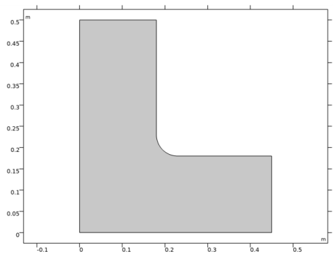
Browse to the model’s Application Libraries folder and double-click the file loaded_knee_geom_sequence.mph.
|
|
3
|
|
4
|
|
1
|
|
2
|
|
3
|
|
4
|
|
5
|
|
2
|
|
3
|
|
4
|
|
1
|
In the Model Builder window, under Component 1 (comp1) right-click Definitions and choose Physics Utilities>Mass Properties.
|
|
2
|
|
3
|
|
1
|
|
2
|
|
3
|
|
4
|
|
1
|
In the Model Builder window, under Component 1 (comp1) right-click Materials and choose More Materials>Topology Link.
|
|
2
|
|
3
|
|
4
|
|
1
|
|
1
|
|
3
|
|
4
|
|
5
|
|
1
|
|
2
|
|
3
|
Click the Custom button.
|
|
4
|
|
5
|
|
1
|
|
1
|
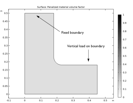
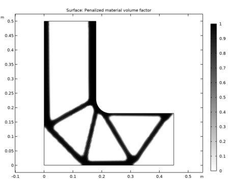
In the Model Builder window, expand the Results>Topology Optimization node, then click Output material volume factor.
|
|
2
|
In the Settings window for 2D Plot Group, type Penalized Material Volume Factor in the Label text field.
|
|
1
|
In the Model Builder window, expand the Penalized Material Volume Factor node, then click Surface 1.
|
|
2
|
In the Settings window for Surface, click Replace Expression in the upper-right corner of the Expression section. From the menu, choose Component 1 (comp1)>Definitions>Density Model 1>Auxiliary variables>dtopo1.theta_p - Penalized material volume factor.
|
|
3
|
|
4
|
|
5
|
|
1
|
|
2
|
|
3
|
In the Settings window for Global Evaluation, click Add Expression in the upper-right corner of the Expressions section. From the menu, choose Component 1 (comp1)>Solid Mechanics>Global>solid.Ws_tot - Total elastic strain energy - J.
|
|
4
|
Click
|
|
1
|
|
2
|
|
1
|
|
2
|
In the Settings window for Global Variable Probe, click Replace Expression in the upper-right corner of the Expression section. From the menu, choose Component 1 (comp1)>Definitions>Density Model 1>Global>dtopo1.theta_avg - Average material volume factor.
|
|
3
|
|
4
|
In the associated text field, type Solid fraction.
|
|
1
|
|
2
|
In the Settings window for Global Variable Probe, click Replace Expression in the upper-right corner of the Expression section. From the menu, choose Component 1 (comp1)>Solid Mechanics>Global>solid.Ws_tot - Total elastic strain energy - J.
|
|
3
|
|
4
|
Select the Description check box.
|
|
5
|
In the associated text field, type Strain energy factor.
|
|
1
|
|
2
|
|
3
|
|
4
|
Click Add Expression in the upper-right corner of the Objective Function section. From the menu, choose Component 1 (comp1)>Definitions>Density Model 1>Global>comp1.dtopo1.theta_avg - Average material volume factor.
|
|
5
|
Click Add Expression in the upper-right corner of the Constraints section. From the menu, choose Component 1 (comp1)>Solid Mechanics>Global>comp1.solid.Ws_tot - Total elastic strain energy - J.
|
|
6
|
Locate the Constraints section. In the table, enter the following settings:
|
|
7
|
|
8
|
|
9
|
|
10
|
|
11
|
|
1
|
|
2
|
|
3
|
Click
|
|
5
|
|
6
|
Click to expand the Advanced Settings section. Select the Reuse solution from previous step check box.
|
|
7
|