PDF

Design Optimization of a Beam
Introduction
When applying design optimization, one has to choose between different techniques with different strengths and weaknesses regarding robustness, learning curve, design freedom and associated potential improvements. This example illustrates how to apply parameter, shape, and topology optimization to the problem of minimizing the weight of a beam subject to a displacement constraint. In this case the parameter and shape optimization happen to give similar designs with similar performance, while the topology optimization gives a design with significantly better performance. Although it is not unusual that the superior design freedom of topology optimization results in superior performance, it is in no way guaranteed. The optimization can get stuck in a local minimum and it is often possible to improve on the result by using it as an initial design for shape or parameter optimization as shown in the model Shape Optimization of a Tesla Microvalve.
Model Definition
The model geometry (Figure 1) consists of two regions: A fixed domain on which a distributed load is applied and a domain to be designed for optimal performance. For the parameter optimization it is the lower right corner that is moved, while the shape optimization changes the bottom right boundary. Finally, topology optimization is able to distribute material freely in the design domain.
Figure 1: The model geometry.
The beam is made of aluminum, and the displacement field is calculated under the assumption of linear elasticity. The displacement of the upper right corner is constrained to be less than 0.2 mm.
The parameter optimization moves the lower right point and constructs a new mesh in every iteration. This means that the gradient cannot be computed analytically using the adjoint method, so the use of a derivative free optimization solver (such as Nelder-Mead) is appropriate.
The shape optimization uses to 2nd order Bernstein polynomials to move the bottom right boundary. This is implemented using the Free Shape Domain and Polynomial Boundary features. The Maximum displacement is set such that the lower boundary cannot move to the point where the topology changes. The lower left point is fixed, but the right point is allowed to slide along a Roller boundary.
For a detailed introduction to the use of structural topology optimization and how to use a Helmholtz filter for regularization, see the model Topology Optimization of an MBB Beam. The main points are that Young’s modulus varies spatially to reflect the material distribution. It is not possible to set zero void stiffness, because this causes the void displacement field to become undefined.
Results and Discussion
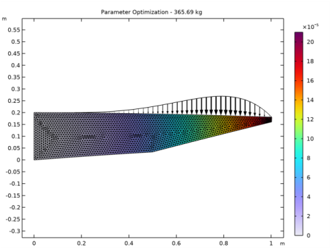
Figure 2 displays the result of the parameter optimization together with the distributed load and the mesh. The displacement field is shown in colors and the maximum value is located near the end of the beam,
Figure 2: The lower right corner is moved to the center of the beam, when its position is used as a control variable. The color scale show reveals that the displacement at the upper right corner satisfies the 0.5 mm constraint.
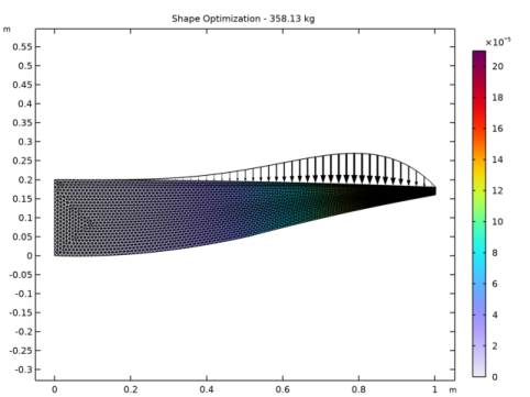
The shape optimization results in a somewhat similar design and the mass is only 1% lower, see Figure 3. However, the study is faster than the parameter optimization despite having more control variables. This is due to the fact that the mesh topology is fixed, which allows for the use of analytic computation of the gradient via the adjoint method. It is thus possible to use IPOPT, a quadratic gradient based optimizer. Moreover, the addition of more control variables is not expected to have affect the computational time adversely.
Figure 3: The shape of the beam is optimized by moving the lower boundary vertically. The movement is large toward the right of the beam, which causes a concentration of elements in this area.
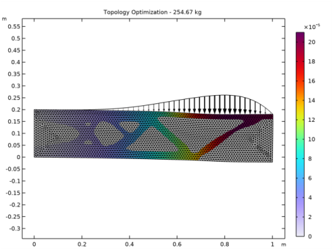
Figure 4 plots the design found with topology optimization. Four triangles have been cut out and the end of the beam is left unsupported, which allows for a seesaw effect because most of the load is to the left of the unsupported region. You can thus expect that the performance of the design is quite sensitive to variations in the load distribution. The model Bracket — Topology Optimization shows how multiple load cases can be used to find design that are robust to load variations.
Figure 4: Topology optimization has significant design freedom, so it is able to find a design, which is 41% lighter than the result of the shape optimization.
Notes About the COMSOL Implementation
This model combines the Optimization and Solid Mechanics interfaces. First, you set up and solve the parameter optimization. Then you define the shape optimization problem using the features available under the component’s Definitions node. Both the shape and parameter optimization work with a coarser mesh, but the topology optimization needs a rather fine mesh if a structure with slender components is desired. This is particularly true, if the constraint on the displacement is relaxed to a higher value.
The topology optimization is implemented by adding a Density Model feature under component definitions. This is used to define a custom Young’s modulus for a new Linear Elasticity model under the Solid Mechanics interface. This new Linear Elasticity model is disabled in the studies for the shape and parameter optimization.
Application Library path: Optimization_Module/Design_Optimization/beam_optimization
Modeling Instructions
From the File menu, choose New.
New
In the New window, click  Model Wizard.
Model Wizard
1
In the Model Wizard window, click  2D.
2
In the Select Physics tree, select Structural Mechanics>Solid Mechanics (solid).
3
Click Add.
4
Click  Study.
5
In the Select Study tree, select General Studies>Stationary.
6
Global Definitions
Parameters 1
Add parameters for the geometry, including the y coordinates for two points to be controlled by the parameter optimization.
1
In the Model Builder window, under Global Definitions click Parameters 1.
2
In the Settings window for Parameters, locate the Parameters section.
3
Geometry 1
Polygon 1 (pol1)
1
In the Geometry toolbar, click  Polygon.
2
In the Settings window for Polygon, locate the Coordinates section.
3
Polygon 2 (pol2)
1
In the Geometry toolbar, click  Polygon.
2
In the Settings window for Polygon, locate the Object Type section.
3
From the Type list, choose Open curve.
4
Locate the Coordinates section. In the table, enter the following settings:
Bottom Boundaries
1
In the Geometry toolbar, click  Selections and choose Box Selection.
2
In the Settings window for Box Selection, type Bottom Boundaries in the Label text field.
3
Locate the Geometric Entity Level section. From the Level list, choose Boundary.
4
Locate the Box Limits section. In the y maximum text field, type eps.
5
Locate the Output Entities section. From the Include entity if list, choose Entity inside box.
Right Boundaries
1
Right-click Bottom Boundaries and choose Duplicate.
2
In the Settings window for Box Selection, type Right Boundaries in the Label text field.
3
Locate the Box Limits section. In the x minimum text field, type L0-eps.
4
In the y maximum text field, type Inf.
5
In the Geometry toolbar, click  Build All.
6
Click the  Zoom Extents button in the Graphics toolbar.
Add Material
1
In the Home toolbar, click  Add Material to open the Add Material window.
2
Go to the Add Material window.
3
In the tree, select Built-in>Aluminum.
4
Click Add to Component in the window toolbar.
5
In the Home toolbar, click  Add Material to close the Add Material window.
Solid Mechanics (solid)
Fix the left boundary. Then impose a nonuniform load on the upper boundary.
Fixed Constraint 1
1
In the Model Builder window, under Component 1 (comp1) right-click Solid Mechanics (solid) and choose Fixed Constraint.
2
Boundary Load 1
1
In the Physics toolbar, click  Boundaries and choose Boundary Load.
2
3
In the Settings window for Boundary Load, locate the Force section.
4
From the Load type list, choose Force per unit length.
5
Specify the FL vector as
Mesh 1
1
In the Model Builder window, under Component 1 (comp1) click Mesh 1.
2
In the Settings window for Mesh, locate the Physics-Controlled Mesh section.
3
From the Element size list, choose Extremely fine.
4
Click  Build All.
Enable Variable Utilities and use it do define a Mass Properties feature.
Definitions
Mass Properties 1 (mass1)
1
In the Model Builder window, under Component 1 (comp1) right-click Definitions and choose Physics Utilities>Mass Properties.
2
In the Settings window for Mass Properties, locate the Density section.
3
From the Density source list, choose From physics interface.
Tip Displacement
1
In the Definitions toolbar, click  Probes and choose Point Probe.
2
In the Settings window for Point Probe, type Tip Displacement in the Label text field.
3
In the Variable name text field, type pnt_disp.
4
Study 1
Step 1: Stationary
1
In the Model Builder window, under Study 1 click Step 1: Stationary.
2
In the Settings window for Stationary, click to expand the Results While Solving section.
3
From the Probes list, choose None.
Solve the model without minimization to generate a plot to update while optimizing.
4
In the Model Builder window, click Study 1.
5
In the Settings window for Study, type Parameter Optimization in the Label text field.
6
In the Home toolbar, click  Compute.
Results
Parameter Optimization
1
In the Settings window for 2D Plot Group, type Parameter Optimization in the Label text field.
2
Click to expand the Title section. From the Title type list, choose Manual.
3
In the Title text area, type Parameter Optimization - eval(mass1.mass) kg.
4
Locate the Plot Settings section. Clear the Plot dataset edges check box.
Surface 1
1
In the Model Builder window, expand the Parameter Optimization node, then click Surface 1.
2
In the Settings window for Surface, locate the Expression section.
3
In the Expression text field, type solid.disp.
4
Click to expand the Range section. Select the Manual color range check box.
5
In the Minimum text field, type 0.
6
In the Maximum text field, type 1.05*maxDisp.
Deformation
1
In the Model Builder window, expand the Surface 1 node, then click Deformation.
2
In the Settings window for Deformation, locate the Scale section.
3
Select the Scale factor check box.
4
Mesh 1
1
In the Model Builder window, right-click Parameter Optimization and choose Mesh.
2
In the Settings window for Mesh, locate the Coloring and Style section.
3
From the Element color list, choose None.
Deformation 1
1
Right-click Mesh 1 and choose Deformation.
2
In the Settings window for Deformation, locate the Scale section.
3
Select the Scale factor check box.
4
Line 1
1
In the Model Builder window, right-click Parameter Optimization and choose Line.
2
In the Settings window for Line, locate the Expression section.
3
In the Expression text field, type 1.
4
Locate the Coloring and Style section. From the Coloring list, choose Uniform.
5
From the Color list, choose Black.
Deformation 1
1
Right-click Line 1 and choose Deformation.
2
In the Settings window for Deformation, click Add Expression in the upper-right corner of the Expression section. From the menu, choose Component 1 (comp1)>Solid Mechanics>Load>solid.F_Ax,solid.F_Ay - Load (spatial frame).
3
Locate the Expression section. In the X component text field, type u.
4
In the Y component text field, type v-1e-8*solid.FperLengthy.
5
Locate the Scale section. Select the Scale factor check box.
6
Arrow Line 1
1
In the Model Builder window, right-click Parameter Optimization and choose Arrow Line.
2
In the Settings window for Arrow Line, locate the Expression section.
3
In the X component text field, type solid.FperLengthx.
4
In the Y component text field, type solid.FperLengthy.
5
Locate the Coloring and Style section. From the Arrow base list, choose Head.
6
Select the Scale factor check box.
7
8
Locate the Arrow Positioning section. In the Number of arrows text field, type 160.
9
Locate the Coloring and Style section. From the Color list, choose Black.
Deformation 1
1
Right-click Arrow Line 1 and choose Deformation.
2
In the Settings window for Deformation, locate the Scale section.
3
Select the Scale factor check box.
4
5
In the Parameter Optimization toolbar, click  Plot.
Parameter Optimization
Setup and compute the solution to the parameter optimization problem.
Optimization
1
In the Study toolbar, click  Optimization and choose Optimization.
2
In the Settings window for Optimization, locate the Optimization Solver section.
3
From the Method list, choose COBYLA.
4
Click Add Expression in the upper-right corner of the Objective Function section. From the menu, choose Component 1 (comp1)>Definitions>Mass Properties 1>comp1.mass1.mass - Mass - kg.
5
Locate the Objective Function section. From the Objective scaling list, choose Initial solution based.
6
Locate the Control Variables and Parameters section. Click  Add twice.
7
8
Click Add Expression in the upper-right corner of the Constraints section. From the menu, choose Component 1 (comp1)>Definitions>comp1.pnt_disp - Tip Displacement - m.
9
Locate the Constraints section. In the table, enter the following settings:
10
Locate the Output While Solving section. Select the Plot check box.
11
From the Probes list, choose None.
12
Locate the Optimization Solver section. Find the Solver settings subsection. From the Keep solutions list, choose Only last.
13
In the Model Builder window, click Parameter Optimization.
14
In the Settings window for Study, locate the Study Settings section.
15
Clear the Generate default plots check box.
16
In the Study toolbar, click  Compute.
Results
Parameter Optimization
Click the  Zoom Extents button in the Graphics toolbar.
Next solve the same problem using shape optimization with a Free Shape Domain and a Polynomial Boundary.
Component 1 (comp1)
Next solve the same problem using shape optimization with a Free Shape Domain and a Polynomial Boundary.
1
In the Definitions toolbar, click  Optimization and choose Shape Optimization>Free Shape Domain.
Shape Optimization
Free Shape Domain 1
1
In the Settings window for Free Shape Domain, locate the Domain Selection section.
2
From the Selection list, choose All domains.
Polynomial Boundary 1
1
In the Definitions toolbar, click  Optimization and choose Shape Optimization>Polynomial Boundary.
2
In the Settings window for Polynomial Boundary, locate the Boundary Selection section.
3
From the Selection list, choose Bottom Boundaries.
4
Locate the Control Variable Settings section. In the dmax text field, type 0.9*T0.
Symmetry/Roller 1
1
In the Definitions toolbar, click  Optimization and choose Shape Optimization>Symmetry/Roller.
2
In the Settings window for Symmetry/Roller, locate the Boundary Selection section.
3
From the Selection list, choose Right Boundaries.
Root
Add a study for the shape optimization and run it before adding the optimization, so that a plot can be generated for visualizing the results while optimizing.
Add Study
1
In the Home toolbar, click  Add Study to open the Add Study window.
2
Go to the Add Study window.
3
Find the Studies subsection. In the Select Study tree, select General Studies>Stationary.
4
Click Add Study in the window toolbar.
5
In the Home toolbar, click  Add Study to close the Add Study window.
Study 2
Step 1: Stationary
1
In the Settings window for Stationary, locate the Results While Solving section.
2
From the Probes list, choose None.
3
In the Model Builder window, click Study 2.
4
In the Settings window for Study, locate the Study Settings section.
5
Clear the Generate default plots check box.
6
In the Label text field, type Shape Optimization.
7
In the Home toolbar, click  Compute.
Results
Shape Optimization
1
In the Model Builder window, right-click Parameter Optimization and choose Duplicate.
2
In the Settings window for 2D Plot Group, type Shape Optimization in the Label text field.
3
Locate the Title section. In the Title text area, type Shape Optimization - eval(mass1.mass) kg.
4
Locate the Data section. From the Dataset list, choose Shape Optimization/Solution 4 (sol4).
Parameter Optimization
Optimization
In the Model Builder window, under Parameter Optimization right-click Optimization and choose Copy.
Shape Optimization
In the Model Builder window, right-click Shape Optimization and choose Paste Optimization.
Optimization
1
In the Settings window for Optimization, locate the Optimization Solver section.
2
From the Method list, choose IPOPT.
3
Locate the Control Variables and Parameters section. Ctrl-click to select table rows 1 and 2.
4
Click  Delete.
5
Locate the Output While Solving section. From the Plot group list, choose Shape Optimization.
6
In the Home toolbar, click  Compute.
Results
Shape Optimization
1
In the Shape Optimization toolbar, click  Plot.
2
Click the  Zoom Extents button in the Graphics toolbar.
Finally, setup a topology optimization problem using the density method. Start by adding the Density Model feature, use it to define a penalized Young’s modulus in a alternative Linear Elastic Material.
Component 1 (comp1)
Finally, setup a topology optimization problem using the density method. Start by adding the Density Model feature, use it to define a penalized Young’s modulus in a alternative Linear Elastic Material.
1
In the Definitions toolbar, click  Optimization and choose Topology Optimization>Density Model.
Topology Optimization
Density Model 1 (dtopo1)
1
2
In the Settings window for Density Model, locate the Control Variable Discretization section.
3
From the Element order list, choose Constant.
Prescribed Material 1
1
In the Definitions toolbar, click  Optimization and choose Topology Optimization>Prescribed Material.
2
Solid Mechanics (solid)
Linear Elastic Material 2
1
In the Physics toolbar, click  Domains and choose Linear Elastic Material.
2
3
In the Settings window for Linear Elastic Material, locate the Linear Elastic Material section.
4
From the E list, choose User defined. In the associated text field, type dtopo1.theta_p*mat1.Enu.E.
It is sufficient to interpolate the Young’s modulus, if the theta_avg variable of the Density Model feature is used as objective function, but we also have to interpolate the density, if we want to continue using the mass computed by the Mass Properties features as objective function. Otherwise the Density Model feature will be unable to change the mass/objective function.
5
From the ρ list, choose User defined. In the associated text field, type mat1.def.rho*dtopo1.theta.
Root
Add a study for the optimization. Follow the (now) usual procedure for creating a plot to be used in the optimization.
Add Study
1
In the Home toolbar, click  Add Study to open the Add Study window.
2
Go to the Add Study window.
3
Find the Studies subsection. In the Select Study tree, select General Studies>Stationary.
4
Click Add Study in the window toolbar.
5
In the Home toolbar, click  Add Study to close the Add Study window.
Topology Optimization
1
In the Model Builder window, click Study 3.
2
In the Settings window for Study, type Topology Optimization in the Label text field.
3
Locate the Study Settings section. Clear the Generate default plots check box.
Step 1: Stationary
1
In the Model Builder window, under Topology Optimization click Step 1: Stationary.
2
In the Settings window for Stationary, locate the Physics and Variables Selection section.
3
In the table, clear the Solve for check box for Deformed geometry (Component 1).
4
Locate the Results While Solving section. From the Probes list, choose None.
5
In the Home toolbar, click  Compute.
Results
Topology Optimization
1
In the Model Builder window, right-click Shape Optimization and choose Duplicate.
2
In the Settings window for 2D Plot Group, type Topology Optimization in the Label text field.
3
Locate the Title section. In the Title text area, type Topology Optimization - eval(mass1.mass) kg.
4
Locate the Data section. From the Dataset list, choose Topology Optimization/Solution 5 (sol5).
Filter 1
1
In the Model Builder window, expand the Topology Optimization node.
2
Right-click Surface 1 and choose Filter.
3
In the Settings window for Filter, locate the Element Selection section.
4
In the Logical expression for inclusion text field, type 0.5<dtopo1.theta.
Shape Optimization
Optimization
In the Model Builder window, under Shape Optimization right-click Optimization and choose Copy.
Topology Optimization
In the Model Builder window, right-click Topology Optimization and choose Paste Optimization.
Optimization
1
In the Settings window for Optimization, locate the Optimization Solver section.
2
From the Method list, choose MMA.
3
Find the Solver settings subsection. In the Maximum number of model evaluations text field, type 100.
Generally there is no point converging topology optimization in a strict sense, because the topology stops changing much earlier.
4
Locate the Control Variables and Parameters section. In the table, clear the Solve for check box for Polynomial Boundary 1.
5
Locate the Output While Solving section. From the Plot group list, choose Topology Optimization.
6
In the Home toolbar, click  Compute.
Results
Topology Optimization
Click the  Zoom Extents button in the Graphics toolbar.
Parameter Optimization
Optimization
Disable the Density Module control variables in the Parameter Optimization and Shape Optimization studies.
1
In the Model Builder window, under Parameter Optimization click Optimization.
2
In the Settings window for Optimization, locate the Control Variables and Parameters section.
3
In the table, clear the Solve for check boxes for Density Model 1 (dtopo1) and Polynomial Boundary 1.
Shape Optimization
Optimization
1
In the Model Builder window, under Shape Optimization click Optimization.
2
In the Settings window for Optimization, locate the Control Variables and Parameters section.
3
In the table, clear the Solve for check box for Density Model 1 (dtopo1).
Parameter Optimization
Step 1: Stationary
1
In the Model Builder window, under Parameter Optimization click Step 1: Stationary.
2
In the Settings window for Stationary, locate the Physics and Variables Selection section.
3
Select the Modify model configuration for study step check box.
4
In the tree, select Component 1 (Comp1)>Topology Optimization.
5
Click  Disable in Solvers.
6
In the tree, select Component 1 (Comp1)>Deformed Geometry.
7
Click  Disable in Solvers.
8
In the tree, select Component 1 (Comp1)>Solid Mechanics (Solid)>Linear Elastic Material 2.
9
Click  Disable.
Shape Optimization
Step 1: Stationary
1
In the Model Builder window, under Shape Optimization click Step 1: Stationary.
2
In the Settings window for Stationary, locate the Physics and Variables Selection section.
3
Select the Modify model configuration for study step check box.
4
In the tree, select Component 1 (Comp1)>Topology Optimization.
5
Click  Disable in Solvers.
6
In the tree, select Component 1 (Comp1)>Solid Mechanics (Solid)>Linear Elastic Material 2.
7
Click  Disable.