Primary Creep Under Nonconstant Load

In this model example, you study the creep behavior of material under nonconstant loading. You model the primary creep using a Norton-Bailey law and study the difference between the time hardening and the strain hardening methods available in COMSOL Multiphysics.

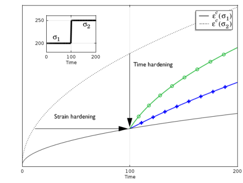
Time hardening assumes that the creep strain rate depends on the current stress and on the time passed from the start of the test. Strain hardening assumes that the creep strain rate depends on the current stress and the accumulated creep strain. Therefore, once the stress level changes, in time hardening the material follows the new behavior from the point where the times are equal, the strain-time relation shifts vertically. In strain hardening, the material follows the new behavior form the point where the strains are equal, the strain-time behavior shifts horizontally. This is illustrated in Figure 1 below.

Figure 1: Strain versus time curve for different primary creep formulations: time hardening in blue(+) and strain hardening in green (o). The load case is represented in the thumbnail in the upper-left corner.

The time hardening formulation is easier to use, while the strain hardening is usually considered to be more accurate.

The model is taken from NAFEMS Understanding Non-Linear Finite Analysis Through Illustrative Benchmarks (Ref. 1). The load consist of a uniaxial and a biaxial stepped load. The step in the load occurs at after a half of the full study time. The value of interest is the creep strain variation along the time. The computed solutions are compared with analytical solution given in the reference.

Additionally, a short discussion describes how to avoid nonphysical creep strains that can appear at the initial time step when a singular load condition is applied at early time.

Model Definition

The problem consists of a 100 mm length square plate under uniaxial and biaxial load cases. Different boundary constraints for each load case ensure uniaxial stress. After 100 hours, the applied load jump from 200 MPa to 250 MPa.

The thickness of the plate is assumed to be small enough to use the 2D plane stress assumption.

The Norton-Bailey that model the creep behavior is represented with the following creep strain definition:

The material constants are listed in the table below:


E	2e5[MPa]
nu	0.3
A	3.125e-14[1/h]
n	5
m	0.5

Both the time hardening and the strain hardening are used to represent the step load response versus time.

Results and Discussion

The problem has analytical results for both uniaxial and biaxial load cases, and for both the time and strain hardening formulations.

For the uniaxial load case, the target solution for the x-component of the creep strain is represented by the following expression:

The target solution for the biaxial load case is represented by the following expression:

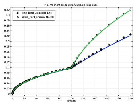
In Figure 2, you can see the results of the computed x-component of the creep strain for the uniaxial load case together with the target data (represented with markers).

Figure 2: The creep strain for time hardening (blue line) and strain hardening (green line) for the uniaxial load case. The reference data is represented by markers.

In the Figure 3, you can see the results of the computed x-component of the creep strain for the biaxial load case together with the target data (represented with markers).

Figure 3: The creep strain for time hardening (blue line) and strain hardening (green line) for the biaxial load case. The reference data is represented by markers.

The computed solutions agree very well with the analytical target for both the uniaxial and the biaxial load cases.

Notes About the COMSOL Implementation

A constant load at the initial time introduces a stress singularity. This can be a source of errors when the strain is defined via a strain rate formulation. At an infinitesimal time step, a nonphysical strain rate can be generated. You can avoid such a singularity by defining the load case using a smooth increase in time. Another solution is to enforce the initial computational time step to be large enough so that the creep strain is reduced. In COMSOL Multiphysics, the time hardening implementation makes it possible to define a time offset. Adjusting the time offset with the initial computational time step ensures to reduce the initial creep strain error. The time should be small compared to the computational study time. In the current example, a time of 1 second as been found sufficient.

For the strain hardening implementation, an initial strain value is requested to avoid an error related to computation a non-integer power of a negative number. Here, a value of 1×10-5 is found to be sufficient.

Reference

1. A.A. Becker, Understanding Non-Linear Finite Element Analysis Through Illustrative Benchmarks, NAFEMS R0080, 2001.

Nonlinear_Structural_Materials_Module/Creep/variable_load_creep

Modeling Instructions

From the menu, choose .

New

In the window, click

Model Wizard

In the window, click

In the tree, select .

Click .

Click

In the tree, select .

Click

Root

In the window, click the root node.

In the root node’s window, locate the section.

From the list, choose .

Global Definitions

Parameters 1

In the window, under click .

In the window for , locate the section.

In the table, enter the following settings:


Name	Expression	Value	Description
A	3.125e-14[1/h]	8.6806E-18 1/s	Creep rate coefficient
n	5	5	Stress exponent
m	0.5	0.5	Power law exponent
t0	1[s]	1 s	Time offset

Definitions

Step 1 (step1)

In the toolbar, click

and choose .

In the window for , type load in the text field.

Locate the section. In the text field, type 100.

In the text field, type 200.

In the text field, type 250.

Global Definitions

Piecewise 1 (pw1)

In the toolbar, click

and choose .

In the window for , type time_hard_uniaxial in the text field.

Locate the section. In the text field, type t.

Find the subsection. In the table, enter the following settings:


Start	End	Function
0	100	0.01*t^0.5
100	200	0.03052*t^0.5-0.2052

Piecewise 2 (pw2)

In the toolbar, click

and choose .

In the window for , type strain_hard_uniaxial in the text field.

Locate the section. In the text field, type t.

Find the subsection. In the table, enter the following settings:


Start	End	Function
0	100	0.01*t^0.5
100	200	0.03052*(t-89.262)^0.5

Piecewise 3 (pw3)

In the toolbar, click

and choose .

In the window for , type time_hard_biaxial in the text field.

Locate the section. In the text field, type t.

Find the subsection. In the table, enter the following settings:


Start	End	Function
0	100	0.005*t^0.5
100	200	0.01529*t^0.5-0.1029

Piecewise 4 (pw4)

In the toolbar, click

and choose .

In the window for , type strain_hard_biaxial in the text field.

Locate the section. In the text field, type t.

Find the subsection. In the table, enter the following settings:


Start	End	Function
0	100	0.005*t^0.5
100	200	0.01529*(t-89.262)^0.5

Geometry 1

Square 1 (sq1)

In the toolbar, click

In the window for , locate the section.

In the text field, type 100[mm].

Click

Click the

button in the toolbar.

Solid Mechanics (solid)

In the window, under click .

In the window for , locate the section.

From the list, choose .

Locate the section. From the list, choose .

Linear Elastic Material 1

In the window, under click .

Creep 1

In the toolbar, click

and choose .

In the window for , locate the section.

Find the subsection. From the h (εce ,t) list, choose .

In the m text field, type m.

In the tshift text field, type t0.

Linear Elastic Material 1

In the window, click .

Creep 2

In the toolbar, click

and choose .

In the window for , locate the section.

Find the subsection. From the h (εce ,t) list, choose .

In the m text field, type m.

Roller 1

In the toolbar, click

and choose .

Select Boundaries 1 and 2 only.

Uniaxial Boundary Load

In the toolbar, click

and choose .

In the window for , type Uniaxial Boundary Load in the text field.

Locate the section. From the list, choose .

Select Boundary 4 only.

Locate the section. Specify the FA vector as


0	t1
load(t[1/h])	n

Biaxial Boundary Load

In the toolbar, click

and choose .

In the window for , type Biaxial Boundary Load in the text field.

Select Boundaries 3 and 4 only.

Locate the section. From the list, choose .

Locate the section. Specify the FA vector as


0	t1
load(t[1/h])	n

Materials

Material 1 (mat1)

In the window, under right-click and choose .

In the window for , locate the section.

In the table, enter the following settings:


Property	Variable	Value	Unit	Property group
Young’s modulus	E	200e3[MPa]	Pa	Young’s modulus and Poisson’s ratio
Poisson’s ratio	nu	0.3	1	Young’s modulus and Poisson’s ratio
Density	rho	0	t/mm³	Basic
Creep rate coefficient	A_nor	A	1/s	Norton
Reference stress	sigRef_nor	1[MPa]	N/m²	Norton
Stress exponent	n_nor	n	1	Norton