You are viewing the documentation for an older COMSOL version. The latest version is available here.
PDF

Two-Stage Powder Compaction Process
Introduction
Powder compaction is a key process in powder metallurgy that allows the manufacturing of quality products of complex shape. The density of the compact is a fundamental factor that determines the overall quality of sintered products, as regions with lower density could reduce the mechanical strength. Multiple parameters and operation conditions are optimized to obtain a uniform density, among these, reducing the friction with the walls and using multistage compaction processes.
This example shows how to setup a two-stage compaction process of metal powder for a simple geometry, and compares the outcome with the results of a single-stage process. The Gurson-Tvergaard-Needleman (GTN) model is used as constitutive model for the porous powder. Friction between the metal powder and the die is taken into account, while perfect bonding between two powder molds is assumed.
Model Definition
The geometry of the workpiece (metal powder) and die are shown in Figure 1. The workpiece geometry is divided into two different domains, for a two-stage compaction process these two domains represent two powder molds at two distinct stages. For the single-stage compaction they represents one powder mold. The punch geometry is not included. Instead, a prescribed displacement at the top boundary is used to compact the powder. Due to the axial symmetry, the geometry can be reduced.
Figure 1: Geometry of the workpiece (metal powder) and die.
Material Properties
The Gurson–Tvergaard–Needleman (GTN) material model is used for the aluminum metal powder. The parameters for the GTN model are given below.
The material of the die is not considered, since it is assumed to be rigid. Hence, the rigid domain model is selected for the die.
Boundary Conditions
The applied boundary conditions are:
Results
Figure 2 shows the volumetric plastic strain at the end of the compaction for two-stage and single-stage processes. For the two-stage process there is layer-wise uniformity in the volumetric plastic strain distribution, while for the single-stage compaction there is a large variation in volumetric plastic strain between the upper and lower boundaries.
Figure 2: Volumetric plastic strain at the end of compaction.
The relative density distribution at the end of the two-stage and single-stage processes are shown in Figure 3 and Figure 4, respectively. The layer-wise uniformity is observed in the relative density for the two-stage process, while for single-stage process there is a clear variation in density from top to bottom. For the two-stage process, the variation in relative density is smaller compared to the single-stage process.
Figure 3: Relative density at the end of compaction for the two-stage process.
Figure 4: Relative density at the end of the compaction for the single-stage process.
The variation of average volumetric elastic strain for the two-stage process is shown in Figure 5. During the first stage of compaction (parameter para between 0 and 1) there is a linear variation of volumetric elastic strain in the first powder mold and no strain in the second one. This is expected as the upper portion of powder is not present in the first stage of compaction. There is elastic rebounding in the first powder mold when the parameter para increases from 1 to 1.1 (punch retraction after first stage of compaction). The second stage of compaction starts when the parameter para reaches the value of 1.1, and ends at the value of 2. In this loading step there is a linear variation in volumetric elastic strains in both powder molds.
Figure 6 shows the punch force versus axial compaction for the two-stage and single-stage processes. The yield point and the end point are almost the same for both cases, but the intermediate states are different. For the two-stage process, there are three stages of punch movement: a first forward movement of the punch on the first powder mold, a retraction of the punch, and finally the forward movement of the punch on the second powder mold. For the single-stage process there is only a forward movement of the punch on the mold.
Figure 5: Variation of average volumetric elastic strain in the two-stage process.
Figure 6: Punch force versus axial compaction.
Notes About the COMSOL Implementation
In the two-stage compaction process analysis the second powder mold is only present during the second stage of compaction. The activation of this mold is performed using the Activation subnode under Linear Elastic Material. Note that the mold will be activated in a stress-free state. The stresses and strains are not considered when the domain is deactivated.
Application Library path: Nonlinear_Structural_Materials_Module/Porous_Plasticity/two_stage_compaction
Modeling Instructions
From the File menu, choose New.
New
In the New window, click  Model Wizard.
Model Wizard
1
In the Model Wizard window, click  2D Axisymmetric.
2
In the Select Physics tree, select Structural Mechanics>Solid Mechanics (solid).
3
Click Add.
4
In the Select Physics tree, select Structural Mechanics>Solid Mechanics (solid).
5
Click Add.
6
Click  Study.
7
In the Select Study tree, select General Studies>Stationary.
8
Model parameters are available in text file.
Global Definitions
Parameters 1
1
In the Model Builder window, under Global Definitions click Parameters 1.
2
In the Settings window for Parameters, locate the Parameters section.
3
Click  Load from File.
4
Punch Force
1
In the Home toolbar, click  Functions and choose Global>Interpolation.
2
In the Settings window for Interpolation, type Punch Force in the Label text field.
3
Locate the Definition section. In the Function name text field, type PunchForce.
4
5
Locate the Units section. In the Argument table, enter the following settings:
6
In the Function table, enter the following settings:
Geometry 1
Rectangle 1 (r1)
1
In the Geometry toolbar, click  Rectangle.
2
In the Settings window for Rectangle, locate the Size and Shape section.
3
In the Width text field, type R0.
4
In the Height text field, type H0.
Rectangle 2 (r2)
1
Right-click Rectangle 1 (r1) and choose Duplicate.
2
In the Settings window for Rectangle, locate the Position section.
3
In the z text field, type H0.
Union 1 (uni1)
1
In the Geometry toolbar, click  Booleans and Partitions and choose Union.
2
Click in the Graphics window and then press Ctrl+A to select both objects.
3
In the Settings window for Union, click  Build Selected.
Rectangle 3 (r3)
1
In the Geometry toolbar, click  Rectangle.
2
In the Settings window for Rectangle, locate the Size and Shape section.
3
In the Width text field, type R0/4.
4
In the Height text field, type 2.5*H0.
5
Locate the Position section. In the r text field, type R0.
6
In the z text field, type -H0/4.
7
Click  Build All Objects.
Form Union (fin)
1
In the Model Builder window, under Component 1 (comp1)>Geometry 1 click Form Union (fin).
2
In the Settings window for Form Union/Assembly, locate the Form Union/Assembly section.
3
From the Action list, choose Form an assembly.
4
From the Pair type list, choose Contact pair.
5
In the Geometry toolbar, click  Build All.
Add a nonlocal integration coupling operator to compute the axial force.
Definitions
Integration 1 (intop1)
1
In the Definitions toolbar, click  Nonlocal Couplings and choose Integration.
2
In the Settings window for Integration, locate the Source Selection section.
3
From the Geometric entity level list, choose Boundary.
4
Integration 2 (intop2)
1
Right-click Integration 1 (intop1) and choose Duplicate.
Add a nonlocal integration coupling operator to compute the axial compaction.
2
In the Settings window for Integration, locate the Source Selection section.
3
Click  Clear Selection.
4
5
Locate the Advanced section. Clear the Compute integral in revolved geometry check box.
Variables 1
1
In the Model Builder window, right-click Definitions and choose Variables.
2
In the Settings window for Variables, locate the Variables section.
3
Setup the both physics interfaces for two-stage compaction and single-stage compaction.
Solid Mechanics (solid)
Linear Elastic Material 1
In the Model Builder window, under Component 1 (comp1)>Solid Mechanics (solid) click Linear Elastic Material 1.
Porous Plasticity 1
1
In the Physics toolbar, click  Attributes and choose Porous Plasticity.
2
In the Settings window for Porous Plasticity, locate the Porous Plasticity Model section.
3
From the Plasticity model list, choose Large plastic strains.
4
From the Yield function F list, choose Gurson-Tvergaard-Needleman.
Linear Elastic Material 1
In the Model Builder window, click Linear Elastic Material 1.
Activation 1
1
In the Physics toolbar, click  Attributes and choose Activation.
2
In the Settings window for Activation, locate the Domain Selection section.
3
Click  Clear Selection.
4
5
Locate the Activation section. In the Activation expression text field, type para>1.
Rigid Domain 1
1
In the Physics toolbar, click  Domains and choose Rigid Domain.
2
Fixed Constraint 1
In the Physics toolbar, click  Attributes and choose Fixed Constraint.
Contact 1
In the Model Builder window, under Component 1 (comp1)>Solid Mechanics (solid) click Contact 1.
Friction 1
1
In the Physics toolbar, click  Attributes and choose Friction.
2
In the Settings window for Friction, locate the Friction Parameters section.
3
In the μ text field, type 0.05.
Prescribed Displacement 1
1
In the Physics toolbar, click  Boundaries and choose Prescribed Displacement.
2
3
In the Settings window for Prescribed Displacement, locate the Prescribed Displacement section.
4
Select the Prescribed in z direction check box.
Boundary Load 1
1
In the Physics toolbar, click  Boundaries and choose Boundary Load.
2
3
In the Settings window for Boundary Load, locate the Force section.
4
From the Load type list, choose Total force.
5
Specify the Ftot vector as
Boundary Load 2
1
Right-click Boundary Load 1 and choose Duplicate.
2
In the Settings window for Boundary Load, locate the Boundary Selection section.
3
Click  Clear Selection.
4
5
Locate the Force section. Specify the Ftot vector as
Solid Mechanics 2 (solid2)
Linear Elastic Material 1
In the Model Builder window, under Component 1 (comp1)>Solid Mechanics 2 (solid2) click Linear Elastic Material 1.
Porous Plasticity 1
1
In the Physics toolbar, click  Attributes and choose Porous Plasticity.
2
In the Settings window for Porous Plasticity, locate the Porous Plasticity Model section.
3
From the Plasticity model list, choose Large plastic strains.
4
From the Yield function F list, choose Gurson-Tvergaard-Needleman.
Rigid Domain 1
1
In the Physics toolbar, click  Domains and choose Rigid Domain.
2
Fixed Constraint 1
In the Physics toolbar, click  Attributes and choose Fixed Constraint.
Contact 1
In the Model Builder window, under Component 1 (comp1)>Solid Mechanics 2 (solid2) click Contact 1.
Friction 1
1
In the Physics toolbar, click  Attributes and choose Friction.
2
In the Settings window for Friction, locate the Friction Parameters section.
3
In the μ text field, type 0.05.
Prescribed Displacement 1
1
In the Physics toolbar, click  Boundaries and choose Prescribed Displacement.
2
3
In the Settings window for Prescribed Displacement, locate the Prescribed Displacement section.
4
Select the Prescribed in z direction check box.
Prescribed Displacement 2
1
Right-click Prescribed Displacement 1 and choose Duplicate.
2
3
In the Settings window for Prescribed Displacement, locate the Prescribed Displacement section.
4
In the u0z text field, type -disp.
Add Material
1
In the Home toolbar, click  Add Material to open the Add Material window.
2
Go to the Add Material window.
3
In the tree, select Built-in>Aluminum.
4
Right-click and choose Add to Component 1 (comp1).
5
In the Home toolbar, click  Add Material to close the Add Material window.
Materials
Aluminum (mat1)
1
In the Settings window for Material, locate the Material Contents section.
2
Mesh 1
Mapped 1
In the Mesh toolbar, click  Mapped.
Distribution 1
1
Right-click Mapped 1 and choose Distribution.
2
3
In the Settings window for Distribution, locate the Distribution section.
4
In the Number of elements text field, type 1.
5
Click  Build All.
Size
1
In the Model Builder window, under Component 1 (comp1)>Mesh 1 click Size.
2
In the Settings window for Size, locate the Element Size section.
3
From the Predefined list, choose Finer.
4
Click  Build All.
Study: Two-Stage Compaction
1
In the Model Builder window, click Study 1.
2
In the Settings window for Study, type Study: Two-Stage Compaction in the Label text field.
Step 1: Stationary
1
In the Model Builder window, under Study: Two-Stage Compaction click Step 1: Stationary.
2
In the Settings window for Stationary, locate the Physics and Variables Selection section.
3
Select the Modify model configuration for study step check box.
4
In the tree, select Component 1 (Comp1)>Solid Mechanics 2 (Solid2).
5
Click  Control Frame Deformation.
6
In the tree, select Component 1 (Comp1)>Solid Mechanics 2 (Solid2).
7
Click  Disable in Solvers.
8
Click to expand the Study Extensions section. Select the Auxiliary sweep check box.
9
10
11
In the Home toolbar, click  Compute.
Add Study
1
In the Home toolbar, click  Add Study to open the Add Study window.
2
Go to the Add Study window.
3
Find the Studies subsection. In the Select Study tree, select General Studies>Stationary.
4
5
In the Home toolbar, click  Add Study to close the Add Study window.
Study: Single-Stage Compaction
1
In the Settings window for Study, type Study: Single-Stage Compaction in the Label text field.
2
Locate the Study Settings section. Clear the Generate default plots check box.
Step 1: Stationary
1
In the Model Builder window, under Study: Single-Stage Compaction click Step 1: Stationary.
2
In the Settings window for Stationary, locate the Physics and Variables Selection section.
3
Select the Modify model configuration for study step check box.
4
In the tree, select Component 1 (Comp1)>Solid Mechanics (Solid).
5
Click  Control Frame Deformation.
6
Click  Disable in Solvers.
7
Locate the Study Extensions section. Select the Auxiliary sweep check box.
8
9
10
In the Home toolbar, click  Compute.
First create the revolution datasets needed to create the plots used in the documentation.
Results
Revolution 2D 2
1
In the Model Builder window, expand the Results>Datasets node.
2
Right-click Results>Datasets>Revolution 2D 1 and choose Duplicate.
3
In the Settings window for Revolution 2D, locate the Data section.
4
From the Dataset list, choose Study: Single-Stage Compaction/Solution 2 (sol2).
Study: Two-Stage Compaction/Solution 1 (3) (sol1)
In the Model Builder window, under Results>Datasets right-click Study: Two-Stage Compaction/Solution 1 (sol1) and choose Duplicate.
Selection
1
In the Results toolbar, click  Attributes and choose Selection.
2
In the Settings window for Selection, locate the Geometric Entity Selection section.
3
From the Geometric entity level list, choose Domain.
4
Revolution 2D 3
1
In the Model Builder window, under Results>Datasets right-click Revolution 2D 1 and choose Duplicate.
2
In the Settings window for Revolution 2D, locate the Data section.
3
From the Dataset list, choose Study: Two-Stage Compaction/Solution 1 (3) (sol1).
Study: Single-Stage Compaction/Solution 2 (4) (sol2)
In the Model Builder window, under Results>Datasets right-click Study: Single-Stage Compaction/Solution 2 (sol2) and choose Duplicate.
Selection
1
In the Results toolbar, click  Attributes and choose Selection.
2
In the Settings window for Selection, locate the Geometric Entity Selection section.
3
From the Geometric entity level list, choose Domain.
4
Revolution 2D 4
1
In the Model Builder window, under Results>Datasets right-click Revolution 2D 2 and choose Duplicate.
2
In the Settings window for Revolution 2D, locate the Data section.
3
From the Dataset list, choose Study: Single-Stage Compaction/Solution 2 (4) (sol2).
Revolution 2D 3, Revolution 2D 4, Study: Single-Stage Compaction/Solution 2 (4) (sol2), Study: Two-Stage Compaction/Solution 1 (3) (sol1)
1
In the Model Builder window, under Results>Datasets, Ctrl-click to select Study: Two-Stage Compaction/Solution 1 (3) (sol1), Revolution 2D 3, Study: Single-Stage Compaction/Solution 2 (4) (sol2), and Revolution 2D 4.
2
Datasets for Die
In the Settings window for Group, type Datasets for Die in the Label text field.
Stress, Two-Stage Compaction
1
In the Model Builder window, under Results click Stress (solid).
2
In the Settings window for 2D Plot Group, type Stress, Two-Stage Compaction in the Label text field.
3
In the Stress, Two-Stage Compaction toolbar, click  Plot.
Stress, Single-Stage Compaction
1
Right-click Stress, Two-Stage Compaction and choose Duplicate.
2
Drag and drop Stress, Two-Stage Compaction 1 below Stress, Two-Stage Compaction.
3
In the Settings window for 2D Plot Group, type Stress, Single-Stage Compaction in the Label text field.
4
Locate the Data section. From the Dataset list, choose Study: Single-Stage Compaction/Solution 2 (2) (sol2).
5
From the Parameter value (disp (mm)) list, choose 6.2.
Surface 1
1
In the Model Builder window, expand the Stress, Single-Stage Compaction node, then click Surface 1.
2
In the Settings window for Surface, locate the Expression section.
3
In the Expression text field, type solid2.misesGp.
Deformation
1
In the Model Builder window, expand the Surface 1 node, then click Deformation.
2
In the Settings window for Deformation, locate the Expression section.
3
In the R component text field, type u2.
4
In the Z component text field, type w2.
Filter 1
In the Model Builder window, under Results>Stress, Single-Stage Compaction>Surface 1 right-click Filter 1 and choose Delete.
Stress, Single-Stage Compaction
1
In the Model Builder window, under Results click Stress, Single-Stage Compaction.
2
In the Stress, Single-Stage Compaction toolbar, click  Plot.
Relative Density, Two-Stage Compaction
1
In the Model Builder window, under Results click Stress, 3D (solid).
2
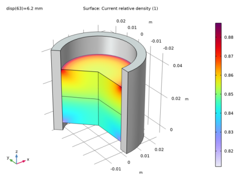
In the Settings window for 3D Plot Group, type Relative Density, Two-Stage Compaction in the Label text field.
Surface 1
1
In the Model Builder window, expand the Relative Density, Two-Stage Compaction node, then click Surface 1.
2
In the Settings window for Surface, click Replace Expression in the upper-right corner of the Expression section. From the menu, choose Component 1 (comp1)>Solid Mechanics>Porous plasticity>solid.lemm1.popl1.rhorel - Current relative density.
Surface 2
1
Right-click Results>Relative Density, Two-Stage Compaction>Surface 1 and choose Duplicate.
2
In the Settings window for Surface, locate the Data section.
3
From the Dataset list, choose Revolution 2D 3.
4
From the Solution parameters list, choose From parent.
5
Locate the Expression section. In the Expression text field, type 1.
6
Click to expand the Title section. From the Title type list, choose None.
7
Locate the Coloring and Style section. From the Coloring list, choose Uniform.
8
From the Color list, choose Gray.
Material Appearance 1
Right-click Surface 2 and choose Material Appearance.
Relative Density, Two-Stage Compaction
In the Relative Density, Two-Stage Compaction toolbar, click  Plot.
Relative Density, Single-Stage Compaction
1
In the Model Builder window, right-click Relative Density, Two-Stage Compaction and choose Duplicate.
2
Drag and drop Relative Density, Two-Stage Compaction 1 below Relative Density, Two-Stage Compaction.
3
In the Settings window for 3D Plot Group, type Relative Density, Single-Stage Compaction in the Label text field.
4
Locate the Data section. From the Dataset list, choose Revolution 2D 2.
5
From the Parameter value (disp (mm)) list, choose 6.2.
Surface 1
1
In the Model Builder window, expand the Relative Density, Single-Stage Compaction node, then click Surface 1.
2
In the Settings window for Surface, locate the Expression section.
3
In the Expression text field, type solid2.lemm1.popl1.rhorel.
Filter 1
1
In the Model Builder window, expand the Surface 1 node.
2
Right-click Results>Relative Density, Single-Stage Compaction>Surface 1>Filter 1 and choose Delete.
Deformation
1
In the Model Builder window, under Results>Relative Density, Single-Stage Compaction>Surface 1 click Deformation.
2
In the Settings window for Deformation, locate the Expression section.
3
In the R component text field, type u2.
4
In the Z component text field, type w2.
Surface 2
1
In the Model Builder window, under Results>Relative Density, Single-Stage Compaction click Surface 2.
2
In the Settings window for Surface, locate the Data section.
3
From the Dataset list, choose Revolution 2D 4.
Filter 1
1
In the Model Builder window, expand the Surface 2 node.
2
Right-click Results>Relative Density, Single-Stage Compaction>Surface 2>Filter 1 and choose Delete.
Deformation
1
In the Model Builder window, under Results>Relative Density, Single-Stage Compaction>Surface 2 click Deformation.
2
In the Settings window for Deformation, locate the Expression section.
3
In the R component text field, type u2.
4
In the Z component text field, type w2.
Relative Density, Single-Stage Compaction
1
In the Model Builder window, under Results click Relative Density, Single-Stage Compaction.
2
In the Relative Density, Single-Stage Compaction toolbar, click  Plot.
Volumetric Plastic Strain
1
In the Model Builder window, under Results click Volumetric Plastic Strain (solid).
2
In the Settings window for 2D Plot Group, type Volumetric Plastic Strain in the Label text field.
3
Locate the Plot Settings section. Clear the Plot dataset edges check box.
Contour 2
1
In the Model Builder window, expand the Volumetric Plastic Strain node.
2
Right-click Results>Volumetric Plastic Strain>Contour 1 and choose Duplicate.
3
In the Settings window for Contour, locate the Data section.
4
From the Dataset list, choose Study: Single-Stage Compaction/Solution 2 (2) (sol2).
5
Locate the Expression section. In the Expression text field, type if(isnan(solid2.epvol),NaN,solid2.epvol).
6
Click to expand the Title section. From the Title type list, choose None.
7
Click to expand the Inherit Style section. From the Plot list, choose Contour 1.
Filter 1
1
In the Model Builder window, expand the Contour 2 node.
2
Right-click Results>Volumetric Plastic Strain>Contour 2>Filter 1 and choose Delete.
Translation 1
1
In the Model Builder window, right-click Contour 2 and choose Translation.
2
In the Settings window for Translation, locate the Translation section.
3
In the y text field, type 50[mm].
Volumetric Plastic Strain
In the Model Builder window, under Results click Volumetric Plastic Strain.
Table Annotation 1
1
In the Volumetric Plastic Strain toolbar, click  More Plots and choose Table Annotation.
2
In the Settings window for Table Annotation, locate the Data section.
3
From the Source list, choose Local table.
4
5
Locate the Coloring and Style section. Clear the Show point check box.
6
In the Volumetric Plastic Strain toolbar, click  Plot.
Void Volume Fraction
1
In the Model Builder window, under Results click Current Void Volume Fraction (solid).
2
In the Settings window for 2D Plot Group, type Void Volume Fraction in the Label text field.
3
Locate the Plot Settings section. Clear the Plot dataset edges check box.
Contour 2
1
In the Model Builder window, expand the Void Volume Fraction node.
2
Right-click Results>Void Volume Fraction>Contour 1 and choose Duplicate.
Deformation
1
In the Model Builder window, expand the Results>Void Volume Fraction>Contour 1 node.
2
Right-click Results>Void Volume Fraction>Contour 1>Deformation and choose Delete.
Contour 2
1
In the Model Builder window, under Results>Void Volume Fraction click Contour 2.
2
In the Settings window for Contour, locate the Data section.
3
From the Dataset list, choose Study: Single-Stage Compaction/Solution 2 (2) (sol2).
4
Locate the Expression section. In the Expression text field, type if(isnan(solid2.f),NaN,solid2.f).
5
Locate the Title section. From the Title type list, choose None.
6
Locate the Inherit Style section. From the Plot list, choose Contour 1.
Filter 1
1
In the Model Builder window, expand the Contour 2 node.
2
Right-click Results>Void Volume Fraction>Contour 2>Filter 1 and choose Delete.
Deformation
In the Model Builder window, right-click Deformation and choose Delete.
Translation 1
1
In the Model Builder window, right-click Contour 2 and choose Translation.
2
In the Settings window for Translation, locate the Translation section.
3
In the y text field, type 50[mm].
Void Volume Fraction
In the Model Builder window, under Results click Void Volume Fraction.
Table Annotation 1
1
In the Void Volume Fraction toolbar, click  More Plots and choose Table Annotation.
2
In the Settings window for Table Annotation, locate the Data section.
3
From the Source list, choose Local table.
4
5
Locate the Coloring and Style section. Clear the Show point check box.
6
In the Void Volume Fraction toolbar, click  Plot.
Create 1D plot of average elastic volumetric strain in the workpiece to understand the elastic rebounding phenomenon in two-stage compaction.
Average Elastic Volumetric Strain, Two-Stage Compaction
1
In the Results toolbar, click  Evaluation Group.
2
In the Settings window for Evaluation Group, type Average Elastic Volumetric Strain, Two-Stage Compaction in the Label text field.
Surface Average 1
1
Right-click Average Elastic Volumetric Strain, Two-Stage Compaction and choose Average>Surface Average.
2
3
In the Settings window for Surface Average, locate the Expressions section.
4
Surface Average 2
1
In the Model Builder window, right-click Average Elastic Volumetric Strain, Two-Stage Compaction and choose Average>Surface Average.
2
3
In the Settings window for Surface Average, locate the Expressions section.
4
Average Elastic Volumetric Strain, Two-Stage Compaction
1
In the Model Builder window, click Average Elastic Volumetric Strain, Two-Stage Compaction.
2
In the Settings window for Evaluation Group, click to expand the Format section.
3
From the Include parameters list, choose Off.
4
In the Average Elastic Volumetric Strain, Two-Stage Compaction toolbar, click  Evaluate.
Average Elastic Volumetric Strain, Two-Stage Compaction
1
In the Home toolbar, click  Add Plot Group and choose 1D Plot Group.
2
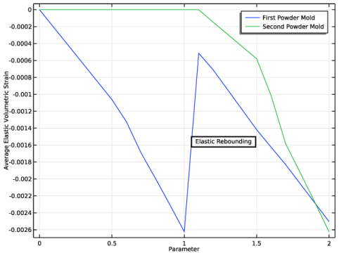
In the Settings window for 1D Plot Group, type Average Elastic Volumetric Strain, Two-Stage Compaction in the Label text field.
3
Locate the Plot Settings section. Select the y-axis label check box.
4
In the associated text field, type Average Elastic Volumetric Strain.
5
Drag and drop below Contact Forces (solid).
Table Graph 1
1
Right-click Average Elastic Volumetric Strain, Two-Stage Compaction and choose Table Graph.
2
In the Settings window for Table Graph, locate the Data section.
3
From the Source list, choose Evaluation group.
4
From the x-axis data list, choose Parameter.
5
Click to expand the Legends section. Select the Show legends check box.
6
From the Legends list, choose Manual.
7
Annotation 1
1
In the Model Builder window, right-click Average Elastic Volumetric Strain, Two-Stage Compaction and choose Annotation.
2
In the Settings window for Annotation, locate the Annotation section.
3
In the Text text field, type Elastic Rebounding.
4
Locate the Position section. In the R text field, type 1.05.
5
In the Z text field, type -0.0015.
6
Locate the Coloring and Style section. Clear the Show point check box.
7
Select the Show frame check box.
8
In the Average Elastic Volumetric Strain, Two-Stage Compaction toolbar, click  Plot.
Create a 1D plot of punch forces for both processes.
Punch Force Vs. Axial Compaction
1
In the Home toolbar, click  Add Plot Group and choose 1D Plot Group.
2
Drag and drop below Average Elastic Volumetric Strain, Two-Stage Compaction.
3
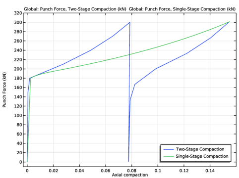
In the Settings window for 1D Plot Group, type Punch Force Vs. Axial Compaction in the Label text field.
4
Locate the Plot Settings section. Select the x-axis label check box.
5
Select the y-axis label check box.
6
7
In the x-axis label text field, type Axial compaction.
8
Locate the Axis section. Select the Manual axis limits check box.
9
In the x minimum text field, type -0.003.
10
In the x maximum text field, type 0.16.
11
In the y minimum text field, type -10.
12
In the y maximum text field, type 320.
13
Locate the Legend section. From the Position list, choose Lower right.
Global 1
1
Right-click Punch Force Vs. Axial Compaction and choose Global.
2
In the Settings window for Global, locate the y-Axis Data section.
3
4
Locate the x-Axis Data section. From the Parameter list, choose Expression.
5
In the Expression text field, type delta.
6
Click to expand the Legends section. From the Legends list, choose Manual.
7
Global 2
1
Right-click Global 1 and choose Duplicate.
2
In the Settings window for Global, locate the Data section.
3
From the Dataset list, choose Study: Single-Stage Compaction/Solution 2 (2) (sol2).
4
Locate the y-Axis Data section. In the table, enter the following settings:
5
Locate the Legends section. In the table, enter the following settings:
6
In the Punch Force Vs. Axial Compaction toolbar, click  Plot.