
|
|
|

|
•
|
A strain rate dependent factor with two parameters (C and
|
|
•
|
A temperature dependent factor for softening. The reference temperature used to define Th is typically the one at which k and n are determined.
|
|
12.3·10-61/K
|
||
|
|
||
|
1
|
|
2
|
In the Select Physics tree, select Structural Mechanics>Thermal-Structure Interaction>Thermal Stress, Solid.
|
|
3
|
Click Add.
|
|
4
|
Click
|
|
5
|
|
6
|
Click
|
|
1
|
|
2
|
|
1
|
|
2
|
|
3
|
|
1
|
|
2
|
|
3
|
|
4
|
|
5
|
|
6
|
|
1
|
|
2
|
|
3
|
|
4
|
|
5
|
|
6
|
|
7
|
|
8
|
|
1
|
|
2
|
Click in the Graphics window and then press Ctrl+A to select both objects.
|
|
3
|
|
1
|
|
2
|
On the object csol1, select Point 5 only.
|
|
3
|
|
4
|
|
5
|
|
1
|
In the Model Builder window, under Component 1 (comp1) right-click Solid Mechanics (solid) and choose More Constraints>Symmetry Plane.
|
|
1
|
|
3
|
|
4
|
|
5
|
|
1
|
|
2
|
|
3
|
|
1
|
|
2
|
|
3
|
|
4
|
|
5
|
|
1
|
|
1
|
|
2
|
|
3
|
|
4
|
|
1
|
In the Model Builder window, under Component 1 (comp1)>Multiphysics click Thermal Expansion 1 (te1).
|
|
2
|
|
3
|
|
4
|
|
5
|
|
6
|
In the Show More Options dialog box, in the tree, select the check box for the node Physics>Advanced Physics Options.
|
|
7
|
Click OK.
|
|
1
|
In the Model Builder window, under Component 1 (comp1)>Solid Mechanics (solid) click Linear Elastic Material 1.
|
|
2
|
|
3
|
|
1
|
|
2
|
|
3
|
|
1
|
|
2
|
|
3
|
|
4
|
|
1
|
|
2
|
|
1
|
|
2
|
|
3
|
Click
|
|
1
|
|
2
|
|
3
|
In the Output times text field, type range(0,0.01*tFinal,0.1*tFinal) range(0.12*tFinal,0.02*tFinal,tFinal).
|
|
1
|
|
2
|
|
3
|
|
4
|
|
5
|
|
1
|
|
2
|
|
3
|
|
1
|
|
2
|
|
3
|
|
1
|
|
2
|
|
3
|
|
4
|
|
1
|
|
2
|
|
3
|
Locate the Data section. From the Dataset list, choose Study 1: With Thermal Softening/Parametric Solutions 1 (sol2).
|
|
1
|
|
3
|
|
4
|
|
5
|
|
6
|
|
7
|
|
8
|
|
9
|
|
10
|
|
11
|
|
1
|
|
2
|
|
3
|
|
4
|
|
5
|
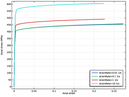
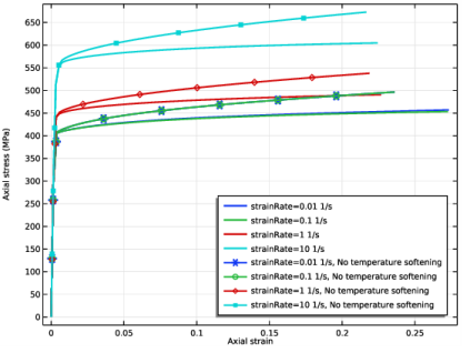
In the associated text field, type Axial strain.
|
|
6
|
|
7
|
In the associated text field, type Axial stress (MPa).
|
|
8
|
|
9
|
|
1
|
|
2
|
|
3
|
|
5
|
|
1
|
|
2
|
|
1
|
|
2
|
|
3
|
Locate the Data section. From the Dataset list, choose Study 1: With Thermal Softening/Parametric Solutions 1 (sol2).
|
|
4
|
|
1
|
|
2
|
|
4
|
|
5
|
|
6
|
|
7
|
|
8
|
|
9
|
Select the Description check box.
|
|
10
|
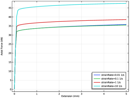
In the associated text field, type Extension.
|
|
11
|
|
12
|
|
1
|
|
2
|
|
3
|
|
4
|
|
1
|
|
2
|
|
3
|
|
4
|
|
5
|
|
1
|
|
2
|
|
3
|
Click
|
|
1
|
|
2
|
|
3
|
In the Output times text field, type range(0,0.01*tFinal,0.1*tFinal) range(0.12*tFinal,0.02*tFinal,tFinal).
|
|
1
|
In the Model Builder window, under Component 1 (comp1)>Solid Mechanics (solid)>Linear Elastic Material 1 right-click Plasticity 1 and choose Duplicate.
|
|
2
|
|
3
|
|
1
|
|
2
|
|
3
|
|
4
|
In the tree, select Component 1 (Comp1)>Solid Mechanics (Solid)>Linear Elastic Material 1>Plasticity 2.
|
|
5
|
Right-click and choose Disable.
|
|
1
|
|
2
|
|
3
|
|
4
|
|
5
|
|
6
|
|
7
|
|
8
|
|
1
|
In the Model Builder window, under Results>Stress vs. Strain right-click Point Graph 1 and choose Duplicate.
|
|
2
|
|
3
|
|
4
|
|
5
|
|
6
|
Locate the Legends section. Find the Prefix and suffix subsection. In the Suffix text field, type , No temperature softening.
|
|
7
|
|
1
|
|
2
|
|
3
|
|
4
|
|
5
|
|
6
|
|
7
|
|
8
|
|
1
|
In the Model Builder window, expand the Equivalent Plastic Strain (solid) node, then click Contour 1.
|
|
2
|
|
3
|
|
4
|
|
5
|
|
1
|
|
2
|
|
3
|
|
4
|
Click to expand the Advanced section. Locate the Display section. From the Display list, choose Max.
|
|
5
|
|
6
|
|
1
|
|
2
|
|
3
|
|
4
|
|
5
|
|
6
|
|
7
|
|
8
|
|
9
|
|
10
|
|
11
|
|
12
|
|
1
|
In the Model Builder window, under Results>Equivalent Plastic Strain (solid), Ctrl-click to select Contour 1, Max/Min Surface 1, and Annotation 1.
|
|
2
|
Right-click and choose Duplicate.
|
|
1
|
|
2
|
|
3
|
|
4
|
|
5
|
|
1
|
|
2
|
|
3
|
|
4
|
|
5
|
|
1
|
|
2
|
|
3
|
|
4
|
|
5
|
|
1
|
In the Model Builder window, under Results>Equivalent Plastic Strain (solid), Ctrl-click to select Contour 2, Max/Min Surface 2, and Annotation 2.
|
|
2
|
Right-click and choose Duplicate.
|
|
1
|
|
2
|
|
1
|
In the Model Builder window, expand the Contour 3 node, then click Results>Equivalent Plastic Strain (solid)>Max/Min Surface 3.
|
|
2
|
|
3
|
|
4
|
|
5
|
|
1
|
In the Model Builder window, expand the Max/Min Surface 3 node, then click Results>Equivalent Plastic Strain (solid)>Annotation 3.
|
|
2
|
|
3
|
|
4
|
|
1
|
In the Model Builder window, under Results>Equivalent Plastic Strain (solid), Ctrl-click to select Contour 3, Max/Min Surface 3, and Annotation 3.
|
|
2
|
Right-click and choose Duplicate.
|
|
1
|
In the Model Builder window, under Results>Equivalent Plastic Strain (solid), Ctrl-click to select Contour 4 and Annotation 4.
|
|
2
|
|
3
|
|
1
|
In the Model Builder window, expand the Results>Equivalent Plastic Strain (solid)>Contour 4 node, then click Results>Equivalent Plastic Strain (solid)>Max/Min Surface 4.
|
|
2
|
|
3
|
|
4
|
|
1
|
In the Model Builder window, expand the Max/Min Surface 4 node, then click Results>Equivalent Plastic Strain (solid)>Annotation 4.
|
|
2
|
|
3
|
|
4
|
|
5
|
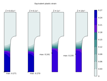
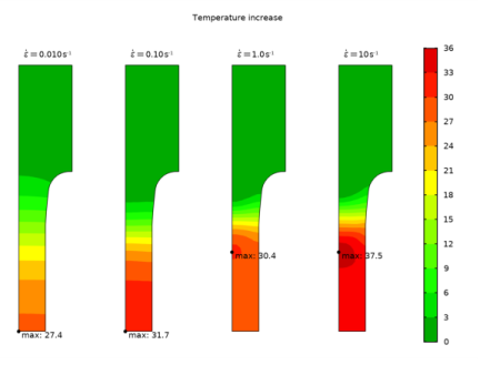
Locate the Annotation section. In the Text text field, type $\dot \varepsilon = eval(strainRate) \; \mathrm s^{-1}$.
|
|
1
|
|
2
|
|
3
|
|
4
|
|
1
|
|
2
|
|
3
|
|
4
|
|
1
|
|
2
|
|
3
|
|
4
|
|
5
|
|
1
|
|
2
|
|
3
|
|
4
|
|
1
|
|
2
|
|
3
|
|
4
|
|
1
|
|
2
|
|
3
|
|
4
|
|
1
|
|
2
|
|
3
|
|
1
|
|
2
|
|
3
|
|
1
|
|
2
|
|
3
|
|
1
|
|
2
|
|
3
|
|
4
|
|
5
|