PDF

Plastic Strain Mapping
Introduction
Mapping of results, such as plastic strains, between dissimilar meshes can be useful in different situations. This model demonstrates a simple and effective way to accomplish this. In the example, you will model a perforated plate subjected to in plane loading. The analysis is performed in two separate studies. In the first study (Study 1), the plate is modeled using triangular mesh elements, and it is loaded well into its plastic regime. The elastoplastic solution at an intermediate stage of deformation is then used as a starting point for a second study (Study 2), where the plastic strains are mapped onto a plate discretized with quadrilateral mesh elements. The results from the two studies are compared after unloading.
Model Definition
Figure 1 shows the plate’s geometry. Due to the double symmetry of the geometry you only need to analyze a quarter of the plate.
Figure 1: The plate geometry.
Because the plate is thin and the loads are in plane, you can assume a plane stress condition.
Material
Elastic properties: E = 70000 MPa and ν = 0.2.
Plastic properties: Yield stress 243 MPa and a linear isotropic hardening with tangent modulus 2171 MPa.
Constraints and loads
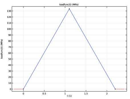
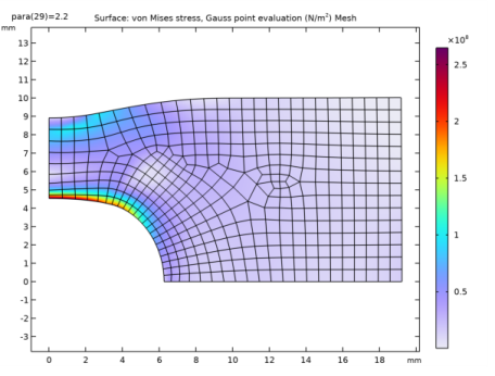
The right vertical edge is subjected to a stress, which increases from zero to a maximum value of 133.65 MPa and then is released. The peak value is selected so that the mean stress over the section through the hole is 10% above the yield stress (=1.1·243·(2010)/20). The complete release of the stress corresponds to a parameter value of 2.2, see Figure 2.
Figure 2: The stress applied to the right vertical edge.
Studies
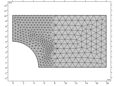
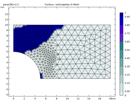
In Study 1, a plate that uses triangular mesh elements is used, see Figure 3. The plate is loaded, and then released using the prescribed stress on the right vertical edge, see Figure 2.
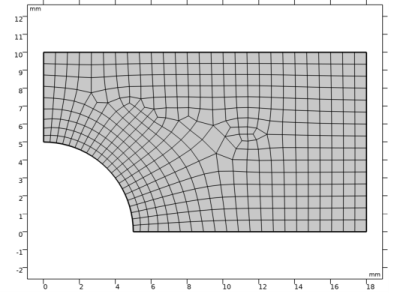
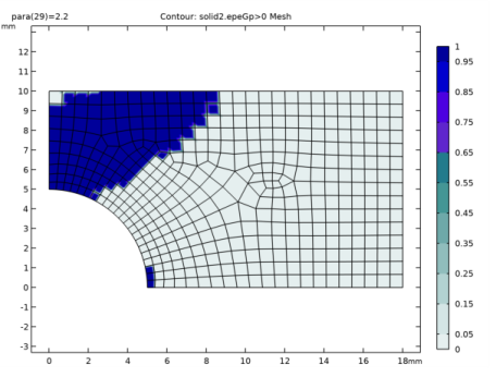
In Study 2, a plate that uses quadrilateral mesh elements is used, see Figure 4. This study is started from an intermediate stage, corresponding to a parameter value of 0.8, see Figure 2. The displacements and plastic strains from the plate in Study 1 are mapped onto the plate in Study 2..
Figure 3: The plate, discretized with triangular mesh elements.
Figure 4: The plate, discretized with quadrilateral mesh elements.
Results and Discussion
Figure 5 and Figure 6 show the von Mises stress distribution after unloading, for the two cases of triangular and quadrilateral meshes. To within the small differences that can be attributed to different mesh element types and differences in mesh topology, the results are the same.
Figure 5: Deformation and von Mises stress after unloading, using the plate with
triangular mesh elements.
Figure 6: Deformation and von Mises stress after unloading, using the plate with quadrilateral mesh elements.
Figure 7 and Figure 8 show the regions where plastic straining has occurred, after unloading, for the two cases of triangular and quadrilateral meshes. In these figures, a value of one means that the equivalent plastic strain is greater than zero, and a value of zero means that the material at that location has deformed purely elastically throughout the process. In this comparison, the differences appear larger, however the differences stem from the discrete (zero to one) character of the output, in combination with the differences in mesh element types and differences in topology.
Figure 7: Plastic region after unloading, using the plate with triangular mesh elements.
Figure 8: Plastic region after unloading, using the plate with quadrilateral mesh elements.
Notes About the COMSOL Implementation
To properly initialize the study of the plate using quadrilateral mesh elements, there are two modeling aspects to consider:
Because the mapping is to be performed between two different components, a general extrusion operator is used. The assignment of plastic strains is performed using the Set Variables subnode to the Plasticity node. With this subnode, you can set plastic variables to certain values, on satisfying a logical condition that you define. The study using quadrilateral elements is performed from an intermediate deformation stage, corresponding to a parameter value para = 0.8, and the logical condition is expressed accordingly.
To properly initialize the second study, the equivalent plastic strain (epe) and the plastic strain tensor (ep) are prescribed.
Application Library path: Nonlinear_Structural_Materials_Module/Plasticity/plastic_strain_mapping
Modeling Instructions
From the File menu, choose New.
New
In the New window, click  Model Wizard.
Model Wizard
1
In the Model Wizard window, click  2D.
2
In the Select Physics tree, select Structural Mechanics>Solid Mechanics (solid).
3
Click Add.
4
Click  Study.
5
In the Select Study tree, select General Studies>Stationary.
6
Geometry 1
Begin by changing the length unit to millimeters.
1
In the Model Builder window, under Component 1 (comp1) click Geometry 1.
2
In the Settings window for Geometry, locate the Units section.
3
From the Length unit list, choose mm.
Rectangle 1 (r1)
1
In the Geometry toolbar, click  Rectangle.
2
In the Settings window for Rectangle, locate the Size and Shape section.
3
In the Width text field, type 18.
4
In the Height text field, type 10.
5
Click  Build Selected.
Circle 1 (c1)
1
In the Geometry toolbar, click  Circle.
2
In the Settings window for Circle, locate the Size and Shape section.
3
In the Radius text field, type 5.
4
Click  Build Selected.
Difference 1 (dif1)
1
In the Geometry toolbar, click  Booleans and Partitions and choose Difference.
2
3
In the Settings window for Difference, locate the Difference section.
4
Find the Objects to subtract subsection. Click to select the  Activate Selection toggle button.
5
6
Click  Build Selected.
Define the elastoplastic material properties.
Global Definitions
Material 1 (mat1)
1
In the Model Builder window, under Global Definitions right-click Materials and choose Blank Material.
2
Expand the Material 1 (mat1) node.
3
In the Model Builder window, under Global Definitions>Materials>Material 1 (mat1) click Basic (def).
4
In the Settings window for Basic, locate the Output Properties section.
5
Click  Select Quantity.
6
In the Physical Quantity dialog box, click  Filter.
7
In the tree, select Solid Mechanics>Young’s modulus (Pa).
8
9
In the Settings window for Basic, locate the Output Properties section.
10
11
Click  Select Quantity.
12
In the Physical Quantity dialog box, select Solid Mechanics>Poisson’s ratio (1) in the tree.
13
14
In the Settings window for Basic, locate the Output Properties section.
15
16
Click  Select Quantity.
17
In the Physical Quantity dialog box, select General>Density (kg/m^3) in the tree.
18
19
In the Settings window for Basic, locate the Output Properties section.
20
21
In the Model Builder window, click Material 1 (mat1).
22
In the Settings window for Material, click to expand the Material Properties section.
23
In the Material properties tree, select Solid Mechanics>Elastoplastic Material.
24
Click  Add to Material.
25
In the Material properties tree, select Solid Mechanics>Elastoplastic Material>Elastoplastic Material Model.
26
Click  Add to Material.
27
In the Model Builder window, under Global Definitions>Materials>Material 1 (mat1) click Elastoplastic material model (ElastoplasticModel).
28
In the Settings window for Elastoplastic Material Model, locate the Output Properties section.
29
Add a solver parameter for controlling the load expression.
Parameters 1
1
In the Model Builder window, under Global Definitions click Parameters 1.
2
In the Settings window for Parameters, locate the Parameters section.
3
Interpolation 1 (int1)
1
In the Home toolbar, click  Functions and choose Global>Interpolation.
2
In the Settings window for Interpolation, locate the Definition section.
3
In the Function name text field, type loadfunc.
4
5
Locate the Units section. In the Argument table, enter the following settings:
6
In the Function table, enter the following settings:
7
The interpolation function defines the load function.
Materials
Material Link 1 (matlnk1)
In the Model Builder window, under Component 1 (comp1) right-click Materials and choose More Materials>Material Link.
Solid Mechanics (solid)
1
In the Settings window for Solid Mechanics, locate the 2D Approximation section.
2
3
Locate the Thickness section. In the d text field, type 10[mm].
Linear Elastic Material 1
In the Model Builder window, under Component 1 (comp1)>Solid Mechanics (solid) click Linear Elastic Material 1.
Plasticity 1
In the Physics toolbar, click  Attributes and choose Plasticity.
Symmetry 1
1
In the Physics toolbar, click  Boundaries and choose Symmetry.
2
Boundary Load 1
1
In the Physics toolbar, click  Boundaries and choose Boundary Load.
2
3
In the Settings window for Boundary Load, locate the Force section.
4
Specify the FA vector as
Mesh 1
Free Triangular 1
1
In the Mesh toolbar, click  Free Triangular.
The mesh should be refined in areas of anticipated high stress and strain gradients.
Refine 1
1
In the Mesh toolbar, click  Modify and choose Refine.
2
In the Settings window for Refine, click to expand the Refine Elements in Box section.
3
Select the Specify bounding box check box.
4
In row x, set Upper bound to 8.
5
In row y, set Upper bound to 10.
6
In the Model Builder window, right-click Mesh 1 and choose Build All.
Study 1
Step 1: Stationary
Set up an auxiliary sweep for the para parameter.
1
In the Model Builder window, under Study 1 click Step 1: Stationary.
2
In the Settings window for Stationary, click to expand the Study Extensions section.
3
Select the Auxiliary sweep check box.
4
5
With these settings, the edge load you defined earlier increases from zero to a maximum value of 133.65 MPa and is then released.
6
In the Home toolbar, click  Compute.
Results
The default plot shows the von Mises stress for the final parameter value.
Stress, Triangular Mesh
1
In the Model Builder window, under Results click Stress (solid).
2
In the Settings window for 2D Plot Group, type Stress, Triangular Mesh in the Label text field.
3
Locate the Plot Settings section. Clear the Plot dataset edges check box.
Mesh 1
Right-click Stress, Triangular Mesh and choose Mesh.
Mesh 1
1
In the Model Builder window, expand the Results>Stress, Triangular Mesh node, then click Mesh 1.
2
In the Settings window for Mesh, locate the Coloring and Style section.
3
From the Element color list, choose None.
Deformation 1
Right-click Mesh 1 and choose Deformation.
Visualize the plastic zone using a Boolean expression solid.epeGp>0; which is 1 in the plastic region and 0 elsewhere.
Plastic Region, Triangular Mesh
1
In the Model Builder window, under Results click Equivalent Plastic Strain (solid).
2
In the Settings window for 2D Plot Group, type Plastic Region, Triangular Mesh in the Label text field.
Contour 1
1
In the Model Builder window, expand the Plastic Region, Triangular Mesh node, then click Contour 1.
2
In the Settings window for Contour, locate the Expression section.
3
In the Expression text field, type solid.epeGp>0.
4
In the Description text field, type solid.epeGp>0.
Mesh 1
1
In the Model Builder window, right-click Plastic Region, Triangular Mesh and choose Mesh.
2
In the Settings window for Mesh, locate the Coloring and Style section.
3
From the Element color list, choose None.
Now, make a second component that will define the same plate, but using quadrilateral mesh elements.
Add Component
In the Model Builder window, right-click the root node and choose Add Component>2D.
Geometry 2
Import the geometry from the first component into the second.
Import 1 (imp1)
1
In the Home toolbar, click  Import.
2
In the Settings window for Import, locate the Import section.
3
From the Source list, choose Geometry sequence.
4
From the Geometry list, choose Geometry 1.
5
Click Import.
Materials
Material Link 2 (matlnk2)
In the Model Builder window, under Component 2 (comp2) right-click Materials and choose More Materials>Material Link.
Add Physics
1
In the Home toolbar, click  Add Physics to open the Add Physics window.
2
Go to the Add Physics window.
3
In the tree, select Structural Mechanics>Solid Mechanics (solid).
4
Click Add to Component 2 in the window toolbar.
5
In the Home toolbar, click  Add Physics to close the Add Physics window.
Solid Mechanics 2 (solid2)
1
In the Settings window for Solid Mechanics, locate the 2D Approximation section.
2
3
Locate the Thickness section. In the d text field, type 10[mm].
Linear Elastic Material 1
In the Model Builder window, under Component 2 (comp2)>Solid Mechanics 2 (solid2) click Linear Elastic Material 1.
Plasticity 1
In the Physics toolbar, click  Attributes and choose Plasticity.
Set Variables 1
In the Physics toolbar, click  Attributes and choose Set Variables.
To be able to map plastic strains from one component to another, a general extrusion operator is used.
Definitions (comp1)
In the Model Builder window, under Component 1 (comp1) click Definitions.
General Extrusion 1 (genext1)
1
In the Definitions toolbar, click  Nonlocal Couplings and choose General Extrusion.
2
In the Settings window for General Extrusion, locate the Destination Map section.
3
In the x-expression text field, type X.
4
In the y-expression text field, type Y.
5
Locate the Source section. From the Source frame list, choose Material  (X, Y, Z).
6
Solid Mechanics 2 (solid2)
Set Variables 1
The Setting condition is phrased so that it is fulfilled only at the start of the second study, when the parameter value is 0.8.
1
In the Model Builder window, under Component 2 (comp2)>Solid Mechanics 2 (solid2)>Linear Elastic Material 1>Plasticity 1 click Set Variables 1.
2
In the Settings window for Set Variables, locate the Set Variables section.
3
In the Setting condition text field, type para<0.8001.
4
In the εpe text field, type comp1.genext1(solid.epe).
5
In the εp table, enter the following settings:
Symmetry 1
1
In the Physics toolbar, click  Boundaries and choose Symmetry.
2
Boundary Load 1
1
In the Physics toolbar, click  Boundaries and choose Boundary Load.
2
3
In the Settings window for Boundary Load, locate the Force section.
4
Specify the FA vector as
Mesh 2
Free Quad 1
In the Mesh toolbar, click  Free Quad.
Size
1
In the Model Builder window, click Size.
2
In the Settings window for Size, locate the Element Size section.
3
From the Predefined list, choose Finer.
Size 1
1
In the Model Builder window, right-click Free Quad 1 and choose Size.
2
In the Settings window for Size, locate the Geometric Entity Selection section.
3
From the Geometric entity level list, choose Boundary.
4
5
Locate the Element Size section. From the Predefined list, choose Extra fine.
6
Click  Build All.
Add Study
1
In the Home toolbar, click  Add Study to open the Add Study window.
2
Go to the Add Study window.
3
Find the Studies subsection. In the Select Study tree, select General Studies>Stationary.
4
Click Add Study in the window toolbar.
5
In the Home toolbar, click  Add Study to close the Add Study window.
Study 2
Step 1: Stationary
1
In the Settings window for Stationary, locate the Physics and Variables Selection section.
2
In the table, clear the Solve for check box for Solid Mechanics (solid).
3
Click to expand the Values of Dependent Variables section. Find the Initial values of variables solved for subsection. From the Settings list, choose User controlled.
4
From the Study list, choose Study 1, Stationary.
5
From the Parameter value (para) list, choose 0.8.
6
Find the Values of variables not solved for subsection. From the Settings list, choose User controlled.
7
From the Method list, choose Solution.
8
From the Study list, choose Study 1, Stationary.
9
From the Parameter value (para) list, choose 0.8.
10
Locate the Study Extensions section. Select the Auxiliary sweep check box.
11
12
13
Click  Compute.
Results
Stress, Quadrilateral Mesh
1
In the Model Builder window, expand the Results>Stress (solid2) node, then click Stress (solid2).
2
In the Settings window for 2D Plot Group, type Stress, Quadrilateral Mesh in the Label text field.
3
Locate the Plot Settings section. Clear the Plot dataset edges check box.
Mesh 1
1
Right-click Stress, Quadrilateral Mesh and choose Mesh.
2
In the Settings window for Mesh, locate the Coloring and Style section.
3
From the Element color list, choose None.
Deformation 1
Right-click Mesh 1 and choose Deformation.
Plastic Region, Quadrilateral Mesh
1
In the Model Builder window, expand the Results>Equivalent Plastic Strain (solid2) node, then click Equivalent Plastic Strain (solid2).
2
In the Settings window for 2D Plot Group, type Plastic Region, Quadrilateral Mesh in the Label text field.
Contour 1
1
In the Model Builder window, click Contour 1.
2
In the Settings window for Contour, locate the Expression section.
3
In the Expression text field, type solid2.epeGp>0.
4
In the Description text field, type solid2.epeGp>0.
Mesh 1
1
In the Model Builder window, right-click Plastic Region, Quadrilateral Mesh and choose Mesh.
2
In the Settings window for Mesh, locate the Coloring and Style section.
3
From the Element color list, choose None.