|
|
|

|
1
|
|
2
|
|
3
|
Click Add.
|
|
4
|
Click
|
|
5
|
|
6
|
Click
|
|
1
|
|
2
|
|
3
|
|
4
|
Browse to the model’s Application Libraries folder and double-click the file arterial_wall_mechanics_parameters.txt.
|
|
1
|
|
2
|
|
3
|
|
4
|
Click
|
|
5
|
Browse to the model’s Application Libraries folder and double-click the file arterial_wall_mechanics_pressure_radius.txt.
|
|
6
|
|
7
|
Click
|
|
8
|
Find the Functions subsection. In the table, enter the following settings:
|
|
9
|
|
10
|
In the Function table, enter the following settings:
|
|
1
|
|
2
|
|
3
|
|
1
|
|
2
|
|
3
|
|
4
|
|
5
|
|
6
|
Click to expand the Layers section. In the table, enter the following settings:
|
|
7
|
|
8
|
|
9
|
|
1
|
|
2
|
In the Settings window for Rotated System, type Rotated System Media Fiber Family 1 in the Label text field.
|
|
3
|
|
4
|
|
5
|
|
1
|
|
2
|
In the Settings window for Rotated System, type Rotated System Media Fiber Family 2 in the Label text field.
|
|
3
|
Locate the Rotation section. Find the Euler angles (Z-X-Z) subsection. In the β text field, type -betaM.
|
|
1
|
|
2
|
In the Settings window for Rotated System, type Rotated System Adventitia Fiber Family 1 in the Label text field.
|
|
3
|
Locate the Rotation section. Find the Euler angles (Z-X-Z) subsection. In the β text field, type betaA.
|
|
1
|
|
2
|
In the Settings window for Rotated System, type Rotated System Adventitia Fiber Family 2 in the Label text field.
|
|
3
|
Locate the Rotation section. Find the Euler angles (Z-X-Z) subsection. In the β text field, type -betaA.
|
|
1
|
In the Model Builder window, under Component 1 (comp1) right-click Materials and choose Blank Material.
|
|
2
|
|
3
|
|
4
|
|
6
|
|
1
|
|
2
|
|
1
|
|
2
|
|
3
|
From the list, choose Quasistatic.
|
|
1
|
|
2
|
In the Settings window for Hyperelastic Material, type Hyperelastic Material (Media) in the Label text field.
|
|
1
|
|
2
|
In the Settings window for Hyperelastic Material, type Hyperelastic Material (Adventita) in the Label text field.
|
|
4
|
Locate the Hyperelastic Material section. From the Compressibility list, choose Incompressible material.
|
|
1
|
|
2
|
|
3
|
|
1
|
|
2
|
|
3
|
Locate the Coordinate System Selection section. From the Coordinate system list, choose Rotated System Media Fiber Family 1 (sys2).
|
|
4
|
|
5
|
|
1
|
|
2
|
|
3
|
Locate the Coordinate System Selection section. From the Coordinate system list, choose Rotated System Media Fiber Family 2 (sys3).
|
|
1
|
|
2
|
|
3
|
Locate the Coordinate System Selection section. From the Coordinate system list, choose Rotated System Adventitia Fiber Family 1 (sys4).
|
|
4
|
|
5
|
|
1
|
|
2
|
|
3
|
Locate the Coordinate System Selection section. From the Coordinate system list, choose Rotated System Adventitia Fiber Family 2 (sys5).
|
|
1
|
|
1
|
|
3
|
|
4
|
|
5
|
|
1
|
|
3
|
|
4
|
|
5
|
|
1
|
|
3
|
|
4
|
|
1
|
|
3
|
|
4
|
|
5
|
|
1
|
|
2
|
|
1
|
|
2
|
|
1
|
|
2
|
|
3
|
|
1
|
|
2
|
|
3
|
|
4
|
Click
|
|
6
|
Click
|
|
8
|
|
9
|
|
1
|
|
2
|
|
3
|
In the Model Builder window, expand the Study 1>Solver Configurations>Solution 1 (sol1)>Stationary Solver 1 node, then click Parametric 1.
|
|
4
|
|
5
|
|
6
|
|
1
|
|
1
|
|
2
|
|
3
|
|
4
|
|
5
|
|
1
|
|
2
|
|
1
|
In the Model Builder window, under Results>Datasets right-click Study 1/Solution 1 (sol1) and choose Duplicate.
|
|
2
|
|
1
|
|
2
|
|
3
|
|
1
|
|
2
|
|
3
|
|
4
|
|
5
|
|
6
|
Click to expand the Advanced section.
|
|
1
|
|
2
|
|
1
|
|
2
|
|
3
|
|
1
|
|
2
|
In the Settings window for Revolution 2D, type Adventitia Sector Revolution in the Label text field.
|
|
3
|
|
4
|
|
5
|
|
1
|
|
2
|
|
1
|
|
2
|
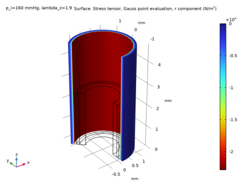
In the Settings window for Surface, click Replace Expression in the upper-right corner of the Expression section. From the menu, choose Component 1 (comp1)>Solid Mechanics>Stress (Gauss points)>Stress tensor, Gauss point evaluation (spatial frame) - N/m²>solid.sGpr - Stress tensor, Gauss point evaluation, r component.
|
|
3
|
|
1
|
|
2
|
|
3
|
|
5
|
|
6
|
|
1
|
|
2
|
|
3
|
|
4
|
|
5
|
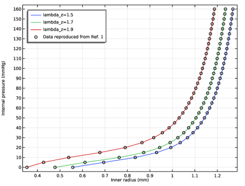
In the associated text field, type Inner radius (mm).
|
|
6
|
|
7
|
In the associated text field, type Internal pressure (mmHg).
|
|
8
|
|
1
|
|
3
|
|
4
|
|
5
|
|
6
|
Click Replace Expression in the upper-right corner of the x-Axis Data section. From the menu, choose Component 1 (comp1)>Geometry>Coordinate (spatial frame)>r - r-coordinate.
|
|
7
|
|
8
|
|
9
|
|
1
|
|
2
|
|
3
|
|
4
|
|
5
|
|
6
|
|
7
|
|
8
|
Click to expand the Coloring and Style section. Find the Line style subsection. From the Line list, choose None.
|
|
9
|
|
10
|
|
11
|
|
12
|
|
1
|
|
2
|
|
3
|
|
4
|
|
1
|
|
2
|
|
3
|
|
4
|
|
1
|
|
2
|
|
3
|
|
4
|
|
1
|
|
2
|
|
3
|
|
4
|
|
5
|
|
6
|
|
7
|
|
8
|
Click Define custom colors.
|
|
10
|
Click Add to custom colors.
|
|
11
|
|
1
|
|
2
|
|
3
|
|
1
|
|
2
|
|
3
|
|
4
|
|
6
|
Click Add to custom colors.
|
|
7
|
|
1
|
|
2
|
|
3
|
|
1
|
|
2
|
|
3
|
|
4
|
|
5
|
|
6
|
|
7
|
|
8
|
|
9
|
Locate the Coloring and Style section. Find the Point style subsection. From the Color list, choose Blue.
|
|
10
|
|
1
|
|
2
|
|
3
|
|
4
|
|
5
|
|
6
|
|
1
|
|
2
|
|
3
|
|
4
|
|
5
|
|
6
|
|
7
|
|
8
|
Locate the Coloring and Style section. Find the Point style subsection. From the Color list, choose Red.
|
|
1
|
|
2
|
|
3
|
|
1
|
|
2
|
|
3
|
|
4
|
|
5
|
|
6
|
|
7
|
|
8
|