PDF

Tuning Fork
Introduction
This example simulates a tuning fork for tuning musical instruments and, if correctly design, should sound the note of A, 440 Hz. It computes the fundamental eigenfrequency and eigenmode for the tuning fork. Although the example seems to be somewhat academic in nature, the eigenfrequencies and eigenmodes of microscopic tuning forks are also used in quartz watches and other electronic devices.
Model Definition
The model geometry is shown in Figure 1. The fundamental frequency of the fork is determined by the length of the prongs, the cross-section geometry of the prongs, and the material properties of the fork.
Figure 1: Tuning fork geometry.
The following formula gives a theoretical estimation for the fundamental frequency of a tuning fork with cylindrical cross section of the prong (Ref. 1):
(1)
where R2 is the radius of the cross section of the prongs, E denotes Young’s modulus, and ρ is the density. The length of the prong can be estimated as
(2)
where R1 the radius of the base, and L is the length of the straight cylindrical part, see Figure 1.
In the fundamental eigenmode, the prongs move according to the figure below. Thus, the eigenmode is symmetric with a symmetry plane placed between the prongs.
The advantage with the shape of the fundamental eigenmode is that the relative displacements in the handle are very small, which makes it possible to hold the fork without damping the vibration. This also allows to make use of the theoretical estimation for the frequency Equation 1 which is based on the solution for a cantilever beam representing each prong.
The parameters used in the model are: R1 = 7.5 mm and R2 = 2.5 mm. The fork material is Steel AISI 4340, for which E = 205 GPa and ρ = 7850 kg/m3.
For the frequency f = 440 Hz, Equation 1 and Equation 2 give the length of the prong cylindrical part as L = 7.8 cm. This presents an underestimation because the part of the prong near the base has larger bending stiffness compared to that for a straight cantilever beam.
To fine-tune the fork, you will use parameterized geometry and gradually increase the cylinder length starting from the above given estimation. To achieve this, you set up a parametric sweep with respect to parameter L.
Reference
1. Tuning fork, https://en.wikipedia.org/wiki/Tuning_fork
Application Library path: COMSOL_Multiphysics/Structural_Mechanics/tuning_fork
Modeling Instructions
From the File menu, choose New.
New
In the New window, click  Model Wizard.
Model Wizard
1
In the Model Wizard window, click  3D.
2
In the Select Physics tree, select Structural Mechanics>Solid Mechanics (solid).
3
Click Add.
4
Click  Study.
5
In the Select Study tree, select General Studies>Eigenfrequency.
6
Global Definitions
Parameters 1
1
In the Model Builder window, under Global Definitions click Parameters 1.
2
In the Settings window for Parameters, locate the Parameters section.
3
Geometry 1
You can build up the fork geometry efficiently using predefined geometry primitives.
Cone 1 (cone1)
1
In the Geometry toolbar, click  Cone.
2
In the Settings window for Cone, locate the Size and Shape section.
3
In the Bottom radius text field, type R2.
4
In the Height text field, type 2e-2.
5
From the Specify top size using list, choose Angle.
6
In the Semiangle text field, type 2.
7
Locate the Position section. In the x text field, type R1.
8
In the z text field, type -R1.
9
Locate the Axis section. From the Axis type list, choose Cartesian.
10
In the z text field, type -1.
Sphere 1 (sph1)
1
In the Geometry toolbar, click  Sphere.
2
In the Settings window for Sphere, locate the Size section.
3
In the Radius text field, type 4e-3.
4
Locate the Position section. In the x text field, type R1.
5
In the z text field, type -(R1+2.25e-2).
Torus 1 (tor1)
1
In the Geometry toolbar, click  Torus.
2
In the Settings window for Torus, locate the Size and Shape section.
3
In the Major radius text field, type R1.
4
In the Minor radius text field, type R2.
5
In the Revolution angle text field, type 180.
6
Locate the Position section. In the x text field, type R1.
7
Locate the Axis section. From the Axis type list, choose Cartesian.
8
In the z text field, type 0.
9
In the y text field, type 1.
10
Locate the Rotation Angle section. In the Rotation text field, type -90.
Union 1 (uni1)
1
In the Geometry toolbar, click  Booleans and Partitions and choose Union.
2
In the Settings window for Union, locate the Union section.
3
Clear the Keep interior boundaries check box.
4
Click in the Graphics window and then press Ctrl+A to select all objects.
This completes the handle and base of the fork.
Add two cylinders to represent the prongs.
Cylinder 1 (cyl1)
1
In the Geometry toolbar, click  Cylinder.
2
In the Settings window for Cylinder, locate the Size and Shape section.
3
In the Radius text field, type R2.
4
In the Height text field, type L.
Cylinder 2 (cyl2)
1
In the Geometry toolbar, click  Cylinder.
2
In the Settings window for Cylinder, locate the Size and Shape section.
3
In the Radius text field, type R2.
4
In the Height text field, type L.
5
Locate the Position section. In the x text field, type 2*R1.
Use virtual geometry operations to avoid short edges and narrow regions. This will improve the mesh generation.
Ignore Edges 1 (ige1)
1
In the Geometry toolbar, click  Virtual Operations and choose Ignore Edges.
2
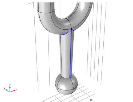
On the object fin, select Edges 22, 23, 29, 32, 33, 39, 42, and 43 only.
It might be easier to select the edges by using the Selection List window. To open this window, in the Home toolbar click Windows and choose Selection List. (If you are running the cross-platform desktop, you find Windows in the main menu.)
3
In the Geometry toolbar, click  Build All.
4
Click the  Go to Default View button in the Graphics toolbar.
The completed geometry should look as shown in the following figure:
Add Material
1
In the Home toolbar, click  Add Material to open the Add Material window.
2
Go to the Add Material window.
3
In the tree, select Built-in>Steel AISI 4340.
4
Click Add to Component in the window toolbar.
5
In the Home toolbar, click  Add Material to close the Add Material window.
Mesh 1
1
In the Model Builder window, under Component 1 (comp1) click Mesh 1.
2
In the Settings window for Mesh, locate the Physics-Controlled Mesh section.
3
From the Element size list, choose Fine.
Free Triangular 1
1
In the Mesh toolbar, click  Boundary and choose Free Triangular.
2
3
In the Settings window for Free Triangular, click  Build Selected.
Swept 1
1
In the Mesh toolbar, click  Swept.
2
In the Settings window for Swept, locate the Domain Selection section.
3
From the Geometric entity level list, choose Domain.
4
Distribution 1
1
Right-click Swept 1 and choose Distribution.
2
In the Settings window for Distribution, locate the Distribution section.
3
In the Number of elements text field, type 50.
Swept 1
In the Model Builder window, right-click Swept 1 and choose Build Selected.
Free Tetrahedral 1
1
In the Mesh toolbar, click  Free Tetrahedral.
2
In the Model Builder window, right-click Mesh 1 and choose Build All.
The meshed geometry should look like that in the figure below.
Study 1
Set up a parametric sweep with respect to the cylinder length L and search for an eigenfrequency in the vicinity of 440 Hz.
Parametric Sweep
1
In the Study toolbar, click  Parametric Sweep.
2
In the Settings window for Parametric Sweep, locate the Study Settings section.
3
4
Step 1: Eigenfrequency
1
In the Model Builder window, click Step 1: Eigenfrequency.
2
In the Settings window for Eigenfrequency, locate the Study Settings section.
3
Select the Desired number of eigenfrequencies check box.
4
5
In the Search for eigenfrequencies around text field, type 440.
Solution 1 (sol1)
1
In the Study toolbar, click  Show Default Solver.
2
In the Model Builder window, expand the Solution 1 (sol1) node, then click Eigenvalue Solver 1.
3
In the Settings window for Eigenvalue Solver, locate the General section.
4
In the Relative tolerance text field, type 1e-3.
5
In the Study toolbar, click  Compute.
Results
To see all computed eigenfrequencies as a table, follow these steps:
Global Evaluation 1
1
In the Results toolbar, click  Global Evaluation.
2
In the Settings window for Global Evaluation, locate the Data section.
3
From the Dataset list, choose Study 1/Parametric Solutions 1 (sol2).
4
From the Table columns list, choose Inner solutions.
5
Click Replace Expression in the upper-right corner of the Expressions section. From the menu, choose Component 1 (comp1)>Solid Mechanics>Global>solid.freq - Frequency - Hz.
6
Clicknext to  Evaluate, then choose New Table.
Table
1
Go to the Table window.
You can see that the eigenfrequency closest to 440 Hz occurs for the cylinder length of 0.0791 m. Further fine-tuning can be performed if necessary.
Results
To see the eigenmode that corresponds to this frequency, do the following:
Mode Shape (solid)
1
In the Model Builder window, under Results click Mode Shape (solid).
2
In the Settings window for 3D Plot Group, locate the Data section.
3
From the Parameter value (L (m)) list, choose 0.0791.
4
In the Mode Shape (solid) toolbar, click  Plot.
5
Click the  Zoom Extents button in the Graphics toolbar.
In this figure, you can clearly see that mode is symmetric, and the displacements at the handle are very small compared to those of the prongs. This means that holding the tuning fork at the handle will dampen the vibrations negligibly.