Rock Fracture Flow

Understanding how fracture flow develops has been an active research area since the 19th century (Ref. 1). The most common model for flow in a single fracture is the so-called “cubic law”, in which the fracture is represented by two parallel plates separated by a small aperture. For the cubic-law assumption, the fluid is considered viscous and incompressible, and the hydraulic conductivity of the fracture depends quadratically on the fracture’s aperture:

which involves the following variables:

•

Fluid density, ρ

•

The acceleration of gravity, g

•

The fluid’s dynamic viscosity, μ

•

The fracture’s aperture or width, a

The transmissivity of the fracture is then proportional to both the hydraulic conductivity and its aperture, giving rise to what is known as the cubic law:

The flux in the fracture is then given by the velocity

which depends on the hydraulic conductivity Ks, the hydraulic head, H = H(x, y), and the hydraulic gradient

. The discharge per unit of fracture width can also be computed from the hydraulic gradient and transmissivity

These expressions are valid as long as the flow is laminar. In cases of deviation from ideal conditions (for instance, rough surfaces) the cubic law can be adjusted by a roughness factor f, so the transmissivity is

A potential flow model describing fluid movement in a rock fracture uses the Reynolds equation

This example uses interpolation data calculated from a fracture with an aperture that changes with position, a(x, y). The data is defined in a text file.

Model Definition

The model consists of two components: the first solves the 2D problem, while the second solves a 3D problem. For the 3D problem, the hydraulic gradient

is given with tangential derivatives.

The computational domain is rectangular. Set a hydraulic head of 20 mm at the upper boundary and 0 mm at the lower boundary. This creates a hydraulic head difference of 20 mm that drives the fluid flow. Both the left and right boundaries are impermeable.

The COMSOL installation includes a text file aperture_data.txt, which contains the sample aperture data in the form of a 100-by-100 matrix. This synthetically generated dataset corresponds to an aperture with a fractal dimension of 2.6. You import the aperture data into the COMSOL Multiphysics physics interface by defining an interpolation function, which you then use as the aperture a(x, y) in the cubic law equation.

Results

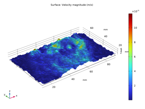
The plot in Figure 1 shows the velocity magnitude using colored surface data and the aperture data as the z-coordinate (the height).

Figure 1: The velocity magnitude and aperture distribution.

The plot in Figure 2 is a visualization of the 3D model.

Figure 2: The velocity magnitude, direction and aperture data in the 3D model.

Notes About the COMSOL Implementation

The base package COMSOL Multiphysics does not include a physics interface that specifically solves for the cubic law, but there are two interfaces under the Mathematics branch you can use: the Convection and Diffusion interface for the 2D model, or the Coefficient Form Boundary PDE for the 3D case. Implement the Reynolds equation by setting the different coefficients for these PDEs. You can rename the dependent variable as H when adding the 2D physics interface, and H2 when adding the 3D physics interface. With a license for the Subsurface Flow Module or Porous Media Flow Module a dedicated interface for modeling fracture flow including the cubic law is available.

Reference

1. P. Witherspoon and others, “Validity of cubic law for fluid flow in a deformable rock fracture,” Lawrence Berkeley National Laboratory. LBNL Paper LBL-9557, 1979.

COMSOL_Multiphysics/Geophysics/rock_fracture_flow

Modeling Instructions

From the menu, choose .

New

In the window, click

Model Wizard

In the window, click

In the tree, select .

Click .

In the text field, type H.

Click

In the dialog box, type head in the text field.

Click

In the tree, select .

Click .

In the window, click

In the dialog box, type timechangeinpressurehead in the text field.

Click

In the tree, select .

Click .

In the window, click

In the tree, select .

Click

Global Definitions

Parameters 1

In the window, under click .

In the window for , locate the section.

In the table, enter the following settings:


Name	Expression	Value	Description
rho	1000[kg/m^3]	1000 kg/m³	Fluid density
mu	0.001[Pa*s]	0.001 Pa·s	Fluid dynamic viscosity

Interpolation 1 (int1)

Define an interpolation function using the aperture data available in a file.

In the toolbar, click

and choose .

In the window for , locate the section.

From the list, choose .

Click

Browse to the model’s Application Libraries folder and double-click the file rock_fracture_flow_aperture_data.txt.

Click

Find the subsection. In the table, enter the following settings:


Function name	Position in file
data	1

Locate the section. In the table, enter the following settings:


Argument	Unit
Argument 1	mm
Argument 2	mm

In the table, enter the following settings:


Function	Unit
data	mm

Click

. Compare with the image below.

Geometry 1

In the window, under click .

In the window for , locate the section.

From the list, choose .

The model geometry is simply a rectangle.

Rectangle 1 (r1)

In the toolbar, click

In the window for , locate the section.

In the text field, type 80.

In the text field, type 50.

Locate the section. In the text field, type 10.

In the text field, type 20.

Click

Definitions

Variables 1

In the window, under right-click and choose .

In the window for , locate the section.

In the table, enter the following settings:


Name	Expression	Unit	Description
a	data(x,y)/1000	m	Aperture
Ks	a^2rhog_const/mu	m/s	Hydraulic conductivity
Ts	Ks*a	m²/s	Transmissivity
u	-Ks*Hx	m/s	Velocity, x component
v	-Ks*Hy	m/s	Velocity, y component
U	sqrt(u^2+v^2)	m/s	Velocity magnitude

Convection-Diffusion Equation (cdeq)

Convection-Diffusion Equation 1

In the window, under click .

In the window for , locate the section.

In the c text field, type Ts.

Locate the section. In the f text field, type 0.

Locate the section. In the da text field, type 0.

Next, define the boundary conditions.

Dirichlet Boundary Condition 1

In the toolbar, click

and choose .

Select Boundary 2 only.

Dirichlet Boundary Condition 2

In the toolbar, click

and choose .

Select Boundary 3 only.

In the window for , locate the section.

In the r text field, type 20[mm].

Mesh 1

In the window, under click .

In the window for , locate the section.

From the list, choose .

Study 1

In the toolbar, click

Results

Velocity (2D)

In the window for , type Velocity (2D) in the text field.

Surface 1

In the window, expand the node, then click .

In the window for , locate the section.

In the text field, type U.

Height Expression 1

Right-click and choose .

In the window for , locate the section.

From the list, choose .

In the text field, type data(x,y).

Locate the section. Select the check box.

In the associated text field, type 1.

In the toolbar, click

Click the

button in the toolbar.

Add Component

In the window, right-click the root node and choose .

Geometry 2

In the window for , locate the section.

From the list, choose .

Parametric Surface 1 (ps1)

In the toolbar, click

and choose .

In the window for , locate the section.

Find the subsection. In the text field, type 10.

In the text field, type 90.

Find the subsection. In the text field, type 20.

In the text field, type 70.

Locate the section. In the text field, type s1.

In the text field, type s2.

In the text field, type data(s1,s2).

Locate the section. In the text field, type 1.0E-2.

In the text field, type 100.

Click

. Compare with the image below.

Definitions (comp2)

Variables 2

In the window, under right-click and choose .

In the window for , locate the section.

In the table, enter the following settings:


Name	Expression	Unit	Description
a	data(x,y)/1000	m	Aperture
Ks	a^2rhog_const/mu	m/s	Hydraulic conductivity
Ts	a*Ks	m²/s	Transmissivity
u	-Ks*H2Tx		Velocity, x component
v	-Ks*H2Ty		Velocity, y component
w	-Ks*H2Tz		Velocity, z component
U	sqrt(u^2+v^2+w^2)		Velocity magnitude