|
|
|


|
-0.5 m4/(mol·s)
|
|
|
1
|
|
2
|
|
3
|
Click Add.
|
|
4
|
|
5
|
Click Add.
|
|
6
|
Click
|
|
7
|
|
8
|
Click
|
|
1
|
|
2
|
|
-0.5 m4/(s·mol)
|
|||
|
-1 m4/(s²·mol)
|
|||
|
-0.001 m4/mol
|
|
1
|
|
2
|
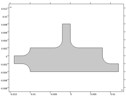
Browse to the model’s Application Libraries folder and double-click the file pid_control_geom_sequence.mph.
|
|
3
|
|
4
|
|
1
|
|
2
|
|
3
|
|
1
|
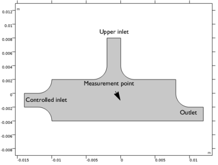
In the Model Builder window, expand the Domain Point Probe 1 node, then click Point Probe Expression 1 (ppb1).
|
|
2
|
|
3
|
Click Replace Expression in the upper-right corner of the Expression section. From the menu, choose Component 1 (comp1)>Transport of Diluted Species>Species c>c - Concentration - mol/m³.
|
|
1
|
|
2
|
|
3
|
|
4
|
|
1
|
In the Add-in Libraries window, in the tree, select the check box for the node COMSOL Multiphysics>pid_controller (if it is not already selected).
|
|
2
|
Click
|
|
1
|
|
2
|
|
4
|
Click Create.
|
|
1
|
In the Model Builder window, under Component 1 (comp1) right-click Materials and choose Blank Material.
|
|
2
|
|
4
|
|
1
|
In the Model Builder window, under Component 1 (comp1) right-click Laminar Flow (spf) and choose Inlet.
|
|
3
|
|
4
|
In the U0 text field, type comp2.u_in_ctrl. This is the inlet velocity defined by the PID controller.
|
|
1
|
|
3
|
|
4
|
|
1
|
|
1
|
|
3
|
|
4
|
|
1
|
In the Model Builder window, under Component 1 (comp1)>Transport of Diluted Species (tds) click Transport Properties 1.
|
|
2
|
|
3
|
|
4
|
|
1
|
|
2
|
|
3
|
|
1
|
|
3
|
|
4
|
|
1
|
|
3
|
|
4
|
|
1
|
|
1
|
|
2
|
|
3
|
|
4
|
|
1
|
|
2
|
|
3
|
Click
|
|
1
|
|
2
|
|
3
|
|
1
|
|
2
|
|
3
|
|
4
|
|
5
|
|
6
|
|
1
|
|
2
|
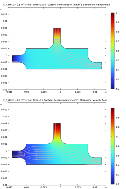
In the Settings window for Streamline, click Replace Expression in the upper-right corner of the Expression section. From the menu, choose Component 1 (comp1)>Laminar Flow>Velocity and pressure>u,v - Velocity field.
|
|
3
|
|
4
|
|
5
|
|
1
|
|
2
|
|
3
|
|
4
|
|
5
|
|
6
|
|
7
|
|
1
|
|
2
|
|
3
|
|
4
|
|
5
|
|
6
|
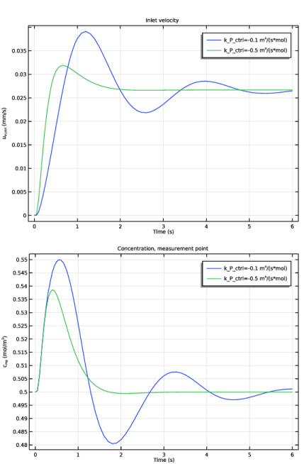
In the associated text field, type u<sub>in,ctrl</sub> (mm/s).
|
|
1
|
|
2
|
In the Settings window for Global, click Replace Expression in the upper-right corner of the y-Axis Data section. From the menu, choose Component 2 (comp2)>Definitions>Variables>comp2.u_in_ctrl - Control variable - m/s.
|
|
3
|
|
4
|
|
1
|
|
2
|
In the Settings window for 1D Plot Group, type Concentration, Measurement Point in the Label text field.
|
|
3
|
|
4
|
Locate the Plot Settings section. In the y-axis label text field, type c<sub>mp</sub> (mol/m<sup>3</sup>).
|
|
1
|
|
2
|
In the Settings window for Global, click Replace Expression in the upper-right corner of the y-Axis Data section. From the menu, choose Component 1 (comp1)>Definitions>c_mp - Domain Point Probe 1, c - mol/m³.
|
|
3
|