PDF

Heat Transfer by Free Convection
Introduction
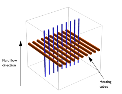
This example describes a fluid flow problem with heat transfer in the fluid. An array of heating tubes is submerged in a vessel with fluid flow entering at the bottom. Figure 1 shows the setup.
Figure 1: Heating tubes and direction of the fluid flow
Model Definition
The first consideration when modeling should always be the true dimension of the problem. Sometimes there are no variations in the third dimensions, and it can be extrapolated from the solution of a related 2D case. By neglecting any end effects from the walls of the vessel, the solution is constant in the direction of the heating tubes. You can therefore reduce the model to a 2D domain.
Figure 2: Using symmetry to reduce computation time and complexity. The model describes one section of the array of heating tubes (indicated by the dashed lines).
The next step is finding symmetries. In this case, using symmetry planes, it suffices to model the thin domain indicated in Figure 2.
Governing Equations
This is a multiphysics model because it involves fluid dynamics coupled with heat transfer. The pressure p and the velocity fields u and v are the solution of the Navier-Stokes equations, while the temperature T is solved through the heat equation. These variables are all related through bidirectional multiphysics couplings.
Results
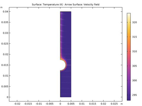
The analysis of the coupled thermal-fluid model provides the velocity field, pressure distribution, and temperature distribution in the fluid. Figure 3 shows a plot of the velocity field and the temperature.
Figure 3: The velocity field and temperature distribution in the fluid.
Using integration to find the mean temperature at the outlet shows that the temperature increases roughly by 1 K from the inlet to the outlet.
Notes About the COMSOL Implementation
To build a model in COMSOL Multiphysics using the above equations, use two physics interfaces: the Laminar Flow interface for laminar single-phase fluid flow and the Heat Transfer in Fluids interface for heat transfer.
In this model, the equations are coupled in both directions. The buoyancy force lifting the fluid is entered in the compressible Navier-Stokes equations via a force term F depending on temperature through the density. At the same time, the heat equation accounts for convective heat transfer.
Use the Nonisothermal Flow multiphysics node to automatically use the temperature field computed in Heat Transfer in Fluids in Laminar Flow and the velocity and pressure from Laminar Flow into Heat Transfer in Fluids.
Application Library path: COMSOL_Multiphysics/Multiphysics/free_convection
Modeling Instructions
From the File menu, choose New.
New
In the New window, click  Model Wizard.
Model Wizard
1
In the Model Wizard window, click  2D.
2
In the Select Physics tree, select Fluid Flow>Single-Phase Flow>Laminar Flow (spf).
3
Click Add.
4
In the Select Physics tree, select Heat Transfer>Heat Transfer in Fluids (ht).
5
Click Add.
6
Click  Study.
7
In the Select Study tree, select General Studies>Stationary.
8
Global Definitions
Parameters 1
1
In the Model Builder window, under Global Definitions click Parameters 1.
2
In the Settings window for Parameters, locate the Parameters section.
3
Geometry 1
Rectangle 1 (r1)
1
In the Geometry toolbar, click  Rectangle.
2
In the Settings window for Rectangle, locate the Size and Shape section.
3
In the Width text field, type 0.005.
4
In the Height text field, type 0.04.
5
Click  Build All Objects.
Circle 1 (c1)
1
In the Geometry toolbar, click  Circle.
2
In the Settings window for Circle, locate the Size and Shape section.
3
In the Radius text field, type 0.0025.
4
Locate the Position section. In the y text field, type 0.015.
5
Click  Build All Objects.
Difference 1 (dif1)
1
In the Geometry toolbar, click  Booleans and Partitions and choose Difference.
2
3
In the Settings window for Difference, locate the Difference section.
4
Find the Objects to subtract subsection. Click to select the  Activate Selection toggle button.
5
6
Click  Build All Objects.
Definitions
Define a nonlocal coupling for computing average values over the outlet.
Average 1 (aveop1)
1
In the Definitions toolbar, click  Nonlocal Couplings and choose Average.
2
In the Settings window for Average, locate the Source Selection section.
3
From the Geometric entity level list, choose Boundary.
4
5
In the Operator name text field, type avgout.
Using this coupling, define a variable, DeltaT, for the temperature rise from inlet to outlet.
Variables 1
1
In the Definitions toolbar, click  Local Variables.
2
In the Settings window for Variables, locate the Variables section.
3
Add Material
1
In the Home toolbar, click  Add Material to open the Add Material window.
2
Go to the Add Material window.
3
In the tree, select Built-in>Water, liquid.
4
Click Add to Component in the window toolbar.
5
In the Home toolbar, click  Add Material to close the Add Material window.
Add a Nonisothermal flow multiphysics node to set up the velocity in heat transfer and to account for the multiphysics stabilization.
Multiphysics
Nonisothermal Flow 1 (nitf1)
In the Physics toolbar, click  Multiphysics Couplings and choose Domain>Nonisothermal Flow.
Laminar Flow (spf)
Since the water density is temperature dependent, the flow is set to weakly compressible.
1
In the Model Builder window, under Component 1 (comp1) click Laminar Flow (spf).
2
In the Settings window for Laminar Flow, locate the Physical Model section.
3
From the Compressibility list, choose Weakly compressible flow.
Symmetry 1
1
In the Physics toolbar, click  Boundaries and choose Symmetry.
2
Inlet 1
1
In the Physics toolbar, click  Boundaries and choose Inlet.
2
3
In the Settings window for Inlet, locate the Velocity section.
4
In the U0 text field, type v_in.
Outlet 1
1
In the Physics toolbar, click  Boundaries and choose Outlet.
2
Initial Values 1
1
In the Model Builder window, click Initial Values 1.
2
In the Settings window for Initial Values, locate the Initial Values section.
3
In the p text field, type spf.rhoref*g_const*(0.04[m]-y).
Volume Force 1
1
In the Physics toolbar, click  Domains and choose Volume Force.
2
3
In the Settings window for Volume Force, locate the Volume Force section.
4
Specify the F vector as
Show advanced physics options as follows, and enable pseudo time stepping for the laminar flow equation for better convergence.
5
Click the  Show More Options button in the Model Builder toolbar.
6
In the Show More Options dialog box, in the tree, select the check box for the node Physics>Advanced Physics Options.
7
8
In the Model Builder window, click Laminar Flow (spf).
9
In the Settings window for Laminar Flow, click to expand the Advanced Settings section.
10
Find the Pseudo time stepping subsection. From the Use pseudo time stepping for stationary equation form list, choose On.
Heat Transfer in Fluids (ht)
In the Model Builder window, under Component 1 (comp1) click Heat Transfer in Fluids (ht).
Temperature 1
1
In the Physics toolbar, click  Boundaries and choose Temperature.
2
3
In the Settings window for Temperature, locate the Temperature section.
4
In the T0 text field, type T_in.
Temperature 2
1
In the Physics toolbar, click  Boundaries and choose Temperature.
2
3
In the Settings window for Temperature, locate the Temperature section.
4
In the T0 text field, type T_heat.
Outflow 1
1
In the Physics toolbar, click  Boundaries and choose Outflow.
2
Symmetry 1
1
In the Physics toolbar, click  Boundaries and choose Symmetry.
2
Initial Values 1
1
In the Model Builder window, click Initial Values 1.
2
In the Settings window for Initial Values, locate the Initial Values section.
3
In the T text field, type T_in.
Mesh 1
In the Model Builder window, under Component 1 (comp1) right-click Mesh 1 and choose Build All.
Study 1
In the Home toolbar, click  Compute.
Results
Temperature (ht)
The default plots visualize the velocity, pressure, and temperature fields. To reproduce the plots in the Figure 3, modify the temperature plot.
Arrow Surface 1
1
In the Model Builder window, right-click Temperature (ht) and choose Arrow Surface.
2
In the Settings window for Arrow Surface, locate the Arrow Positioning section.
3
Find the x grid points subsection. In the Points text field, type 10.
4
Locate the Coloring and Style section. From the Color list, choose White.
5
In the Temperature (ht) toolbar, click  Plot.
6
Click the  Zoom Extents button in the Graphics toolbar.
Finally, evaluate the temperature rise.
Global Evaluation 1
1
In the Results toolbar, click  Global Evaluation.
2
In the Settings window for Global Evaluation, click Replace Expression in the upper-right corner of the Expressions section. From the menu, choose Component 1 (comp1)>Definitions>Variables>DeltaT - Temperature rise - K.
3
Click  Evaluate.
Table
1
Go to the Table window.
The value should be close to 1 K.