PDF

Buoyancy Flow of Free Fluids
Introduction
This example follows the benchmark buoyancy flow posed by de Vahl Davis (Ref. 1) for free fluids. Buoyancy flow of free fluids is very important in Earth sciences with temperature and concentration affecting density in moving fluids, for example, in pipes, along shorelines, and within lakes. Here the buoyancy flow results from density that varies with a temperature change. The COMSOL Multiphysics results match those from the published study (Ref. 1). The model was provided by John Kamel of the University of Notre Dame.
This example repeatedly solves a problem of buoyant flow in a square cavity. It thereby analyzes different temperature distributions and convective flow patterns from variations in, for example, fluid properties, cavity size, and temperature drops. The iterative process is tuned for a fast, efficient solution using nondimensional parameters and a Boussinesq term for the buoyant drive with the Laminar Flow and the Heat Transfer in Fluids interfaces. As an alternative, the same problem can be solved using only the Non-Isothermal Flow interface available with the CFD Module or the Heat Transfer Module.
Figure 1: Domain geometry and boundary conditions for the heat balance in this example of buoyant flow in free fluids.
Model Definition
The previous figure illustrates the model geometry. The fluid fills a square cavity with impermeable walls so the fluid flows freely within it but does not exit from it. The right and left edges of the cavity are, respectively, the high and low temperature sources. The upper and lower boundaries are insulated. The temperature differential produces the density variation that drives the buoyant flow.
The laminar flow and heat transfer interfaces in this example are bidirectionally coupled. The Boussinesq term defines a force dependent on the temperature and the fluid velocity transports heat.
It is possible to formulate the incompressible Navier–Stokes equations with a Boussinesq buoyancy term on the right-hand side to account for the lifting force due to thermal expansion:
In these expressions, the dependent variables for flow are u, the vector of fluid velocity, and pressure, p. T represents temperature, T0 is a reference temperature, g denotes gravity acceleration, ρ0 gives the reference density, μ is the dynamic viscosity, and αp equals the coefficient of volumetric thermal expansion.
The heat balance comes from the conduction-convection equation
where k denotes the thermal conductivity, and Cp is the specific heat capacity of the fluid.
For the Navier–Stokes equations, impermeable, no-slip boundary conditions apply. The no-slip condition results in zero velocity at the wall, with pressure within the domain remaining undefined. Because the lack of information about p makes it difficult to achieve convergence, you arbitrarily fix the pressure at a point.
The boundary conditions for the heat transfer interface are the fixed high and low temperatures on the vertical walls, with insulation conditions elsewhere, as shown in Figure 1.
Notes About the COMSOL Implementation
The model addresses a wide range of cavity sizes, fluid properties, and temperature drops using material properties set up with nondimensional Rayleigh and Prandtl numbers. The Rayleigh number, Ra = (Cpρ2gαpTL3) ⁄ (μk), gives the ratio of buoyant to viscous forces. Here L is the length of a side wall. The Prandtl number, Pr = (μCp ⁄ k), gives the ratio of kinematic viscosity to thermal diffusivity.
Setting the body force in the y-direction for the momentum equation to Fy = (Ra ⁄ Pr)(T − Tc), and the fluid properties to Cp = Pr, and ρ =μ = k = 1, produces a set of equations with nondimensional variables p, u, and T.
As Ra increases, viscous forces decrease in importance. You can examine a wide range of scenarios sequencing through different values of Ra using an Auxiliary sweep with continuation selected for the Ra parameter in the Stationary study step. At high Ra values, starting with a good initial condition and a well-tuned mesh becomes increasingly important. Because the continuation feature in the parametric solver uses extrapolation from the previous solution as the initial condition for the next one, together with automatic step length control, it fulfills the first of these two requirements. Then getting a well-tuned mesh is straightforward: simply set up the mesh for the most difficult problem to solve — the one with the highest value of Ra. To that end, the element size near the prescribed temperature boundaries corresponds to the thickness of the boundary layer when Ra = 106.
Results and Discussion
As noted earlier, this COMSOL Multiphysics example reproduces a benchmark buoyant flow problem reported in Ref. 1. The composite images in Figure 2 summarize temperatures (surface), velocity fields (arrows), and x-velocities (contours) for four Ra values. With the given definitions for the dimensionless variable, it follows that as Ra increases so does temperature. The results in the figure indicate how the vigor and complexity of the convection increase at higher values of Ra, as expected. These results are virtually identical to the benchmark solution except the COMSOL Multiphysics plots provide higher resolution than the images in the original publication.
 
Figure 2: Dimensionless solution for buoyancy flow in a fluid-filled cavity at increasing Raleigh number: Temperature (surface plot), velocity field (arrows), and x-velocity (contours). These results from the COMSOL Multiphysics simulation are in excellent agreement with the results published in Ref. 1.
The COMSOL Multiphysics model described here represents the buoyant drive with a Boussinesq term. As an alternative, you could use the non-isothermal flow interface provided with the laminar flow interface. Using the Boussinesq approach, however, demonstrates a well-established method for reducing computational effort while still representing buoyant flow.
References
1. G. de Vahl Davis and I.P. Jones, “Natural Convection in a Square Cavity: A Comparison Exercise,” Int. J. Num. Meth. in Fluids, vol. 3, pp. 227–248, 1983.
2. G. de Vahl Davis, “Natural Convection of Air in a Square Cavity: A Bench Mark Numerical Solution,” Int. J. Num. Meth. in Fluids, vol. 3, pp. 249–264, 1983.
Application Library path: COMSOL_Multiphysics/Fluid_Dynamics/buoyancy_free
Modeling Instructions
From the File menu, choose New.
New
In the New window, click  Model Wizard.
Model Wizard
1
In the Model Wizard window, click  2D.
2
In the Select Physics tree, select Fluid Flow>Single-Phase Flow>Laminar Flow (spf).
3
Click Add.
4
In the Select Physics tree, select Heat Transfer>Heat Transfer in Fluids (ht).
5
Click Add.
6
Click  Study.
7
In the Select Study tree, select General Studies>Stationary.
8
Global Definitions
Parameters 1
1
In the Model Builder window, under Global Definitions click Parameters 1.
2
In the Settings window for Parameters, locate the Parameters section.
3
Geometry 1
Square 1 (sq1)
1
In the Geometry toolbar, click  Square.
2
In the Settings window for Square, click  Build All Objects.
3
Click the  Zoom Extents button in the Graphics toolbar.
Laminar Flow (spf)
Fluid Properties 1
1
In the Model Builder window, under Component 1 (comp1)>Laminar Flow (spf) click Fluid Properties 1.
2
In the Settings window for Fluid Properties, locate the Fluid Properties section.
3
From the ρ list, choose User defined. In the associated text field, type 1.
4
From the μ list, choose User defined. In the associated text field, type 1.
Initial Values 1
1
In the Model Builder window, click Initial Values 1.
2
In the Settings window for Initial Values, locate the Initial Values section.
3
In the p text field, type p0.
Volume Force 1
1
In the Physics toolbar, click  Domains and choose Volume Force.
2
In the Settings window for Volume Force, locate the Volume Force section.
3
Specify the F vector as
Pressure Point Constraint 1
1
In the Physics toolbar, click  Points and choose Pressure Point Constraint.
2
3
In the Settings window for Pressure Point Constraint, locate the Pressure Constraint section.
4
In the p0 text field, type p0.
Volume Force 1
1
In the Model Builder window, click Volume Force 1.
2
In the Settings window for Volume Force, locate the Domain Selection section.
3
From the Selection list, choose All domains.
Heat Transfer in Fluids (ht)
Fluid 1
1
In the Model Builder window, under Component 1 (comp1)>Heat Transfer in Fluids (ht) click Fluid 1.
2
In the Settings window for Fluid, locate the Model Input section.
3
From the pA list, choose User defined. In the associated text field, type p0.
4
Locate the Heat Convection section. From the u list, choose Velocity field (spf).
5
Locate the Heat Conduction, Fluid section. From the k list, choose User defined. In the associated text field, type 1.
6
Locate the Thermodynamics, Fluid section. From the Fluid type list, choose Gas/Liquid.
7
From the ρ list, choose User defined. In the associated text field, type 1.
8
From the γ list, choose User defined. From the Cp list, choose User defined. In the associated text field, type Pr.
Initial Values 1
1
In the Model Builder window, click Initial Values 1.
2
In the Settings window for Initial Values, locate the Initial Values section.
3
In the T text field, type Tc.
Temperature 1
1
In the Physics toolbar, click  Boundaries and choose Temperature.
2
3
In the Settings window for Temperature, locate the Temperature section.
4
In the T0 text field, type Tc.
Temperature 2
1
In the Physics toolbar, click  Boundaries and choose Temperature.
2
3
In the Settings window for Temperature, locate the Temperature section.
4
In the T0 text field, type Th.
Mesh 1
1
In the Model Builder window, under Component 1 (comp1) click Mesh 1.
2
In the Settings window for Mesh, locate the Physics-Controlled Mesh section.
3
From the Element size list, choose Extra fine.
Edge 1
1
In the Mesh toolbar, click  Edge.
2
Size 1
1
Right-click Edge 1 and choose Size.
2
In the Settings window for Size, locate the Element Size section.
3
From the Predefined list, choose Extremely fine.
Free Triangular 1
1
In the Mesh toolbar, click  Free Triangular.
2
In the Settings window for Free Triangular, click  Build All.
Study 1
Step 1: Stationary
Set up an auxiliary continuation sweep for the Ra parameter.
1
In the Model Builder window, under Study 1 click Step 1: Stationary.
2
In the Settings window for Stationary, click to expand the Study Extensions section.
3
Select the Auxiliary sweep check box.
4
5
6
In the Home toolbar, click  Compute.
Results
Velocity (spf)
The first default plot group shows the velocity magnitude. Notice the high velocities near the lateral walls due to buoyancy effects.
Pressure (spf)
The second default plot group shows the pressure distribution. Because the cavity is closed, the pressure distribution is solely due to gravity.
Temperature (ht)
The third default plot group shows the temperature field as a surface plot. Add arrow and contour plots of the velocity field.
Arrow Surface 1
1
In the Model Builder window, expand the Results>Temperature (ht) node.
2
Right-click Temperature (ht) and choose Arrow Surface.
3
In the Settings window for Arrow Surface, locate the Coloring and Style section.
4
Select the Scale factor check box.
5
6
From the Color list, choose Black.
7
In the Temperature (ht) toolbar, click  Plot.
Contour 1
1
In the Model Builder window, right-click Temperature (ht) and choose Contour.
2
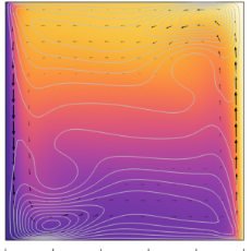
In the Settings window for Contour, click Replace Expression in the upper-right corner of the Expression section. From the menu, choose Component 1 (comp1)>Laminar Flow>Velocity and pressure>Velocity field - m/s>u - Velocity field, x component.
3
Locate the Coloring and Style section. From the Coloring list, choose Uniform.
4
From the Color list, choose Gray.
5
Clear the Color legend check box.
Buoyancy
1
Right-click Temperature (ht) and choose Rename.
2
In the Rename 2D Plot Group dialog box, type Buoyancy in the New label text field.
3
4
In the Settings window for 2D Plot Group, locate the Data section.
5
From the Parameter value (Ra) list, choose 1000.
6
In the Buoyancy toolbar, click  Plot.
Repeat the previous steps for the parameters 1e4, 1e5, and 1e6 to reproduce the remaining plots in Figure 2.