Optimization of a Tesla Microvalve

A Tesla valve inhibits backward flow on a fixed geometry by utilizing friction forces instead of moving parts, Ref. 1. This means fluid can flow freely in one direction but not in the reverse direction. Typically the Reynolds number of the flow in microfluidics is between 1 and 100.

Model Definition

The model solves two instances of the Navier-Stokes equations, one for the forward flow and one for the reverse. The Reynolds number is 100 in this example. A measure of the effectiveness of the design is the ratio of the pressure drop between the inlet and outlet for the forward and reverse flow. The pressure drop is defined as:

For the reverse flow the same expression is used, except the inlet and outlet correspond to different boundaries in the model. The ratio of the pressure drop between the reverse and forward flow is then:

Unfortunately this expression does not form a well posed objective function, so an alternative expression is required for the optimization problem. According to Ref. 2, the energy dissipation is a well posed objective function for topological optimization:

where τ is the viscous stress and S is the strain rate tensor:

The fluid flow is described by the Navier-Stokes equations:

where the coefficient α(θ) depends on the distribution of material which impedes the flow within the device. In this example, α(θ) is given by:

where θc and θf, θ and θp are the control- and filtered material volume factor. To avoid the effect of grayscale the filtered field is projected to construct the material volume factor, θ, which is related to the damping term using a convex function, see Ref. 3. This method is used to avoid grayscale and spurious holes as seen in Figure 1.

Figure 1: Optimizing without a filter gives a design with interpretation issues.

Results and Discussion

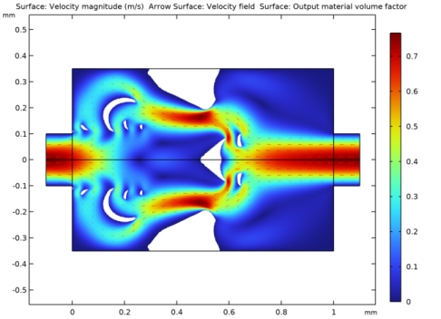
As expected, the forward and reverse flow are identical but in opposite directions for the initial topology; see Figure 2 and Figure 3. The forward flow in the optimized design after 200 iterations can be seen in Figure 4. Material has been added close to the outlet in a triangular shape that makes the forward flow bend smoothly around it. This smooth diversion of the flow from the point of impingement results in an overall low pressure drop between the inlet and the outlet. The reverse flow, shown in Figure 5, is far more interesting. The triangular shaped obstacle has a flat edge normal to the incident fluid, which means the velocity is redirected upward and downward toward the exterior walls. The redirected flow is then directed toward additional obstacles that further impede the flow path.

Figure 2: Forward flow velocity field, initial geometry.

Figure 3: Reverse flow velocity field, initial geometry.

Figure 4: Forward flow, optimized topology.

Figure 5: Reverse flow, optimized topology.

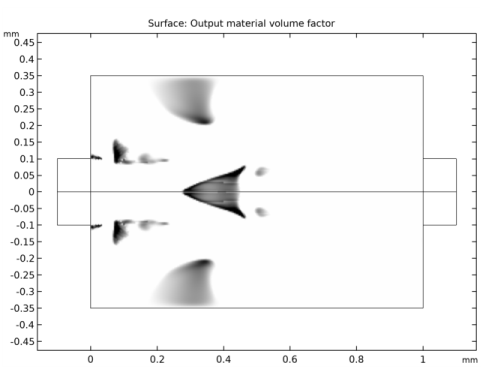
Figure 6: Control variable after optimization.

Finally, the optimized results is transferred to a new component for verification. This results in a larger diodicity.

References

1. S. Lin, “Topology Optimization of Micro Tesla Valve in low and moderate Reynolds number,” Chinese Academy of Sciences, China, September 27, 2011 http://senlin.weebly.com/uploads/6/6/1/4/6614199/sen_lin_topology_optimization_of_micro_tesla_valve.pdf.

2. L. Højgaard Olesen, F. Okkels, and H. Bruus, “A high-level programming-language implementation of topology optimization applied to steady-state Navier–Stokes flow,” Int. J. Numer. Meth. Engng, vol. 65, pp. 975–1001, 2006.

3. T. Borrvall and J. Petersson, “Topology optimization of fluids in Stokes flow,” Int. J. Numer. Meth. Fluid, vol. 41, pp. 77–107, 2003.

Notes About the COMSOL Implementation

The model is set up using two Laminar Flow interfaces, one for the forward flow and one for the reverse. The original MMA optimization solver (which is not globally convergent) is used.

Microfluidics_Module/Fluid_Flow/tesla_microvalve_optimization

Modeling Instructions

From the menu, choose .

New

In the window, click

Model Wizard

In the window, click

In the tree, select .

Add two interfaces, one for the forward flow and one for the backward flow.

Click .

In the tree, select .

Click .

Click

In the tree, select .

Click

Geometry 1

The geometry is on the order of millimeters, so change the geometry unit.

In the window, under click .

In the window for , locate the section.

From the list, choose .

Add some parameters to compute the average inlet velocity for the flow, based on a chosen Reynolds number, in this case, 100.

Global Definitions

Parameters 1

In the window, under click .

In the window for , locate the section.

In the table, enter the following settings:


Name	Expression	Value	Description
Re	100	100	Reynolds number
D	0.2[mm]	2E-4 m	Characteristic dimension
L	5*D	0.001 m	Length of channel
H	1.75*D	3.5E-4 m	Width of channel
mu0	1E-3[Pa*s]	0.001 Pa·s	Dynamic viscosity
rho0	1E3[kg/m^3]	1000 kg/m³	Density
Uin	Remu0/(rho0D)	0.5 m/s	Average inlet velocity
meshsz	0.005*L	5E-6 m	Mesh size

Geometry 1

Rectangle 1 (r1)

In the toolbar, click

In the window for , locate the section.

In the text field, type L.

In the text field, type H.

Rectangle 2 (r2)

In the toolbar, click

In the window for , locate the section.

In the text field, type D/2.

Locate the section. In the text field, type -D/2.

Click

Rectangle 3 (r3)

In the toolbar, click

In the window for , locate the section.

In the text field, type D/2.

Locate the section. In the text field, type L.

Symmetry

In the toolbar, click

and choose .

In the window for , type Symmetry in the text field.

Locate the section. From the list, choose .

Locate the section. In the text field, type 1e3*eps.

Locate the section. From the list, choose .

Left

In the toolbar, click

and choose .

In the window for , type Left in the text field.

Locate the section. From the list, choose .

Locate the section. In the text field, type -D/2+1e3*eps.

Locate the section. From the list, choose .

Right

In the toolbar, click

and choose .

In the window for , type Right in the text field.

Locate the section. From the list, choose .

Locate the section. In the text field, type L+D/2-1e3*eps.

Locate the section. From the list, choose .

Click

Click the

button in the toolbar.

Global Definitions

Add a blank material for rho0 and mu0.

Material 1 (mat1)

In the window, under right-click and choose .

In the toolbar, click

In the window for , locate the section.

Click

In the dialog box, type density in the text field.

Click

In the tree, select .

Click .

In the window for , locate the section.

In the table, enter the following settings:


Property	Variable	Expression	Unit	Size
Density	rho	rho0	kg/m³	1x1

Click

In the dialog box, type viscosity in the text field.

Click

In the tree, select .

Click .

In the window for , locate the section.

In the table, enter the following settings:


Property	Variable	Expression	Unit	Size
Dynamic viscosity	mu	mu0	Pa·s	1x1

Materials

Material Link 1 (matlnk1)

In the window, under right-click and choose .

Laminar Flow (spf)

Inlet 1

In the window, under right-click and choose .

In the window for , locate the section.

From the list, choose .

Locate the section. From the list, choose .

Locate the section. In the Uav text field, type Uin.

Outlet 1

In the toolbar, click

and choose .

In the window for , locate the section.

From the list, choose .

Wall 2

In the toolbar, click

and choose .

In the window for , locate the section.

From the list, choose .

Locate the section. From the list, choose .

Laminar Flow 2 (spf2)

In the window, under click .

Inlet 1

In the toolbar, click

and choose .

In the window for , locate the section.

From the list, choose .

Locate the section. From the list, choose .

Locate the section. In the Uav text field, type Uin.

Outlet 1

In the toolbar, click

and choose .

In the window for , locate the section.

From the list, choose .

Wall 2

In the toolbar, click

and choose .

In the window for , locate the section.

From the list, choose .

Locate the section. From the list, choose .

Mesh 1

In the window, under click .

In the window for , locate the section.

From the list, choose .

Free Triangular 1

In the toolbar, click

Size

In the window, click .

In the window for , click to expand the section.

Locate the section. Click the button.

Locate the section. In the text field, type meshsz.

Click

Study 1

In the toolbar, click

Results

Mirror 2D 1

In the toolbar, click

and choose .

In the window for , locate the section.

In row , set to 1 and to 0.

Velocity (spf)

In the window, under click .

In the toolbar, click

Click the

button in the toolbar.

Velocity (spf2)

In the window, click .

In the toolbar, click

Now define two average operators on the inlet and outlet of the modeling domain. These will be used to compute the pressure ratio between the inlet and outlet for the forward and reverse flow.

Definitions

Average 1 (aveop1)

In the toolbar, click

and choose .

In the window for , locate the section.

From the list, choose .

Average 2 (aveop2)

In the toolbar, click

and choose .

In the window for , locate the section.

From the list, choose .

Integration 1 (intop1)

In the toolbar, click

and choose .

Select Domain 2 only.

Define the variable corresponding to the ratio of the pressure difference between the forward and backward flow.

Variables 1

In the toolbar, click

In the window for , locate the section.

In the table, enter the following settings:


Name	Expression	Unit	Description
dP_forward	aveop1(p)-aveop2(p)	Pa	Pressure difference, forward direction
dP_backward	aveop2(p2)-aveop1(p2)	Pa	Pressure difference, backward direction
Di	dP_backward/dP_forward		Ratio of pressure differences

In order to evaluate the ratio of the pressure differences, the model needs updating. Note that the model does not need to be solved again.

Study 1

In the toolbar, click

Results

Diodicity

In the toolbar, click

In the window for , type Diodicity in the text field.

Global Evaluation 1

Right-click and choose .

In the window for , click in the upper-right corner of the section. From the menu, choose .

In the toolbar, click

Table

Go to the window.

Observe that the ratio of the pressure differences is very close to 1. This concludes solving of the forward problem, now the optimization problem needs to be set up.

Add a density topology feature, which can be used to distinguish between free flow and solid regions. This variable will be coupled back to the interfaces later. The filter radius should not be smaller than the mesh element size, so the default will work, but a fixed value has to be chosen to make the result of the optimization mesh independent.

Definitions

In the toolbar, click

and choose .

Topology Optimization

Density Model 1 (dtopo1)

Only the center part of the channel geometry is needed in the optimization, so you only have to define the feature there.

Select Domain 2 only.

We use a filter to prevent the checkboard instability for the control variable theta which may otherwise occur.

In the window for , locate the section.

From the list, choose .

Locate the section. From the list, choose .

Locate the section. In the qDarcy text field, type 1.

Locate the section. In the θ0 text field, type 1.

Locate the section. From the list, choose .

Now the design variable used in the optimization is defined. The initial value 1 corresponds to a channel free from porous material.

Now define the friction force to be used in the interfaces, the viscous and friction dissipation which can be integrated over the domain to obtain a suitable objective function.

Definitions

Variables 1

In the window, under click .

In the window for , locate the section.

In the table, enter the following settings:


Name	Expression	Unit	Description
phi_forward	spf.Qvd+alpha*(u^2+v^2)	W/m³	Dissipation density, forward flow
phi_backward	spf2.Qvd+alpha*(u2^2+v2^2)	W/m³	Dissipation density, backward flow
phi_total	phi_backward+phi_forward	W/m³	Total dissipation
E_forward	intop1(phi_forward)	W/m	Energy dissipation, forward flow
E_backward	intop1(phi_backward)	W/m	Energy dissipation, backward flow
obj	E_backward/E_forward		Objective function
alpha	16.mu0dtopo1.theta_p/meshsz^2	Pa·s/m²	Friction force