PDF

Lamella Mixer
Introduction
At the macroscopic level, systems usually mix fluids using mechanical actuators or turbulent 3D flow. At the microscale level, however, neither of these approaches is practical or even possible. This model demonstrates the mixing of fluids using laminar-layered flow in a microfluidic mixer.
To characterize the fluid flow’s turbulent behavior scientists generally use the Reynolds number
where ρ is the fluid density, u is flow velocity, L is a characteristic length, and μ is the fluid’s dynamic viscosity. Turbulent flow takes place when the Reynolds number is high, typically when Re > 2000. At microfluidic scales, the width of a channel is in the range of 100 μm and the velocity is approximately 1 cm/s. In this case, for water-like substances Re is close to unity. The fluid flow is thus clearly laminar, so effective mixing of fluids in microfluidic devices requires other means.
Figure 1 shows a section of a component that uses layered flow to improve mixing. The mixer has several lamellae of microchannels, and the two fluids being mixed are alternated for every second layer. Pressure forces the fluid to travel in the channels from back to front. The fluid enters a larger space, the mixing chamber (visible at the front of the image). The figure does not include this chamber, but it covers the area beyond where the grid of the microchannel ends. Near the ends of the microchannels the mixing chamber has distinct lamellae of the two fluids, but this separation vanishes toward the end of the chamber.
Figure 1: Geometry of a lamella mixer (mixing chamber not visible).
Model Definition
This model analyzes the steady-state condition of the fluid flow as well as the convection and diffusion of a dissolved substance in a lamella mixer. The geometry in Figure 2 corresponds to Figure 1 except it includes only a small vertical section of the mixer with a height of 30 μm. The model starts from a plane in the middle of the channel bending to the left and ends at a plane in the middle of the channel bending to the right.
Each microchannel in the mixer has a quadratic cross section with a side of 20 μm. Because of the chosen geometry, microchannel height in the model is only 10 μm. The fluid exiting the microchannels enters a mixing chamber of length 200 μm and width 80 μm.
Figure 2: The model geometry for a lamella mixer takes advantage of symmetry so it is not necessary to model the entire height of the device.
You solve the fluid flow in the channels and in the chamber with the incompressible Navier-Stokes equations
(1)
where ρ is fluid density, u = (u, v, w) is the flow-velocity field, p is fluid pressure, I is the unit diagonal matrix, μ is the fluid’s dynamic viscosity, and F = (fx, fy, fz) is a volume force affecting the fluid. The fluid is water with ρ = 1000 kg/m3, μ = 0.001 Pa·s, and F = 0 because there are no volume forces.
The system applies a pressure of p0 = 10 Pa on all six microchannel inputs to drive the flow through the mixing chamber to where there is zero pressure. At the chamber exit the flow velocity has components only in the normal direction of the boundary.
On the microchannel and mixing-chamber walls, the no slip boundary condition applies. However, in the vertical direction, due to the geometry, you can use a symmetry boundary condition.
The following convection-diffusion equation describes the concentration of the dissolved substances in the fluid:
(2)
where c is the concentration, D is the diffusion coefficient, and R is the reaction rate. In this model, D = 1010 m2/s, and R 0 because the concentration is not affected by any reactions.
There is a concentration of c0 = 50 mol/m3 on the input boundaries of the channels curving to the left, whereas the channels curving to the right have zero concentration. At the output boundary of the mixing chamber the substance flows through the boundary by convection. The walls of the channels and the chamber are insulated for this dissolved substance, and on the top and bottom boundaries you use a symmetry boundary condition.
Results and Discussion
Figure 3 details fluid flow in the mixer. You can see a gradual change in the velocity magnitude across the slices, indicating a laminar parabolic flow. The streamlines do not show swirls, and there are only small changes in the flow direction. The figure also shows that the maximum flow velocity in the microchannels is at the model’s symmetry boundaries. Inside the mixing chamber, a flow velocity gradient is visible only along the x direction; the symmetry conditions on the top and bottom boundaries give a uniform velocity profile in the z direction.
The peak velocity is roughly 1.3 mm/s in the microchannels and 0.6 mm/s in the mixing chamber. Given the corresponding lengths (20 μm and 80 μm), the Reynolds numbers are Re = 0.026 and Re = 0.048, so the flow is clearly laminar.
Figure 3: Fluid flow in the lamella mixer.
Figure 4 shows the concentration distribution on the model boundaries. The inflow channels see a constant concentration of 0 or 50 mol/m3 depending on the channel. Mixing starts when the fluid enters the mixing chamber. At the entrance there is a clear separation of the concentration, but this diminishes toward the end of the chamber. On the sides of the mixing chamber where the flow velocity is smaller the mixing is better than at its center. The mixing, however, is not perfect, and a reduced flow velocity, a longer mixing chamber, or some other means to increase mixing is preferable.
Figure 4: Concentration plot on the boundaries of the lamella mixer model.
To get another point of view, examine Figure 5, which shows the concentration profile at the chamber’s centerline. Near the channels the transition is very rapid, but closer to the chamber’s end the profile has a flatter sigmoid shape. On the chamber’s sides the concentration profile has the same shape, but its amplitude is between approximately 17  mol/m3 and 32 mol/m3.
If you generalize the concentration profile to cover the entire component (Figure 1), the profile would be a wave-like curve where concentration would alternate between its minimum and maximum values with a spatial frequency related to the layer thickness.
Figure 5: Concentration profile along a line in the z direction in the middle of the mixing chamber at various distances from the microchannels: 20 μm (solid), 80 μm (dotted), 140 μm (dashed), and 200 μm (dash-dotted).
Notes About the COMSOL Implementation
Because the concentration does not affect the fluid flow, it is not necessary to solve the Laminar Flow and Transport of Diluted Species interfaces simultaneously. By solving them sequentially, starting with the Navier-Stokes equations, you improve the solution’s convergence and reduce the solution time.
Application Library path: Microfluidics_Module/Micromixers/lamella_mixer
Modeling Instructions
From the File menu, choose New.
New
In the New window, click  Model Wizard.
Model Wizard
1
In the Model Wizard window, click  3D.
2
In the Select Physics tree, select Chemical Species Transport>Reacting Flow>Laminar Flow, Diluted Species.
3
Click Add.
4
Click  Study.
5
In the Select Study tree, select General Studies>Stationary.
6
Geometry 1
For convenience, the device geometry is inserted from an existing file. You can read the instructions for creating the geometry in the Appendix — Geometry Instructions.
1
In the Geometry toolbar, click Insert Sequence and choose Insert Sequence.
2
3
In the Geometry toolbar, click  Build All.
The dimensions of this geometry are given in micrometers, so check the length unit and change it accordingly if necessary.
Global Definitions
Parameters 1
1
In the Model Builder window, under Global Definitions click Parameters 1.
2
In the Settings window for Parameters, locate the Parameters section.
3
Next, add a material for the fluid.
Add Material
1
In the Home toolbar, click  Add Material to open the Add Material window.
2
Go to the Add Material window.
3
In the tree, select Built-in>Water, liquid.
4
Click Add to Component in the window toolbar.
5
In the Home toolbar, click  Add Material to close the Add Material window.
Materials
Water, liquid (mat1)
You are now ready to set up the physics.
Laminar Flow (spf)
Inlet 1
1
In the Model Builder window, under Component 1 (comp1) right-click Laminar Flow (spf) and choose Inlet.
2
In the Settings window for Inlet, locate the Boundary Selection section.
3
From the Selection list, choose Inlet.
4
Locate the Boundary Condition section. From the list, choose Pressure.
5
Locate the Pressure Conditions section. In the p0 text field, type p0.
Symmetry 1
1
In the Physics toolbar, click  Boundaries and choose Symmetry.
2
Click the  Wireframe Rendering button in the Graphics toolbar.
3
In the Settings window for Symmetry, locate the Boundary Selection section.
4
From the Selection list, choose Symmetry.
5
Click the  Zoom Extents button in the Graphics toolbar.
Outlet 1
1
In the Physics toolbar, click  Boundaries and choose Outlet.
2
In the Settings window for Outlet, locate the Boundary Selection section.
3
From the Selection list, choose Outlet.
There are two options available for the type of crosswind diffusion used to provide numerical stabilization. The default option, Do Carmo and Galeao is more effective at suppressing undershoots and overshoots in the concentration, whereas the second option, Codina produces less artificial diffusion in the crosswind direction.
Transport of Diluted Species (tds)
1
Click the  Show More Options button in the Model Builder toolbar.
2
In the Show More Options dialog box, in the tree, select the check box for the node Physics>Stabilization.
3
4
In the Model Builder window, under Component 1 (comp1) click Transport of Diluted Species (tds).
5
In the Settings window for Transport of Diluted Species, click to expand the Consistent Stabilization section.
6
From the Crosswind diffusion type list, choose Codina.
Transport Properties 1
1
In the Model Builder window, under Component 1 (comp1)>Transport of Diluted Species (tds) click Transport Properties 1.
2
In the Settings window for Transport Properties, locate the Diffusion section.
3
In the Dc text field, type D_i.
Note that the velocity field for the species convection is controlled by the Reacting Flow, Diluted Species multiphysics coupling.
Concentration 1
1
In the Physics toolbar, click  Boundaries and choose Concentration.
2
In the Settings window for Concentration, locate the Boundary Selection section.
3
From the Selection list, choose Concentration 1.
4
Locate the Concentration section. Select the Species c check box.
5
In the c0,c text field, type c0.
Concentration 2
1
In the Physics toolbar, click  Boundaries and choose Concentration.
2
In the Settings window for Concentration, locate the Boundary Selection section.
3
From the Selection list, choose Concentration 2.
4
Locate the Concentration section. Select the Species c check box.
Leave the concentration at its default zero value.
Outflow 1
1
In the Physics toolbar, click  Boundaries and choose Outflow.
2
In the Settings window for Outflow, locate the Boundary Selection section.
3
From the Selection list, choose Outlet.
4
Click the  Wireframe Rendering button in the Graphics toolbar.
Mesh 1
Free Tetrahedral 1
In the Mesh toolbar, click  Free Tetrahedral.
Size
1
In the Model Builder window, click Size.
2
In the Settings window for Size, locate the Element Size section.
3
From the Calibrate for list, choose Fluid dynamics.
4
From the Predefined list, choose Fine.
5
Click  Build All.
Study 1
In the Home toolbar, click  Compute.
Results
The following instructions show how to reproduce the plots in the Results and Discussion section.
Slice
1
In the Model Builder window, expand the Velocity (spf) node, then click Slice.
2
In the Settings window for Slice, locate the Plane Data section.
3
From the Plane list, choose zx-planes.
Streamline 1
1
In the Model Builder window, right-click Velocity (spf) and choose Streamline.
2
In the Settings window for Streamline, locate the Streamline Positioning section.
3
From the Positioning list, choose Magnitude controlled.
4
In the Min distance text field, type 0.01.
5
In the Max distance text field, type 0.025.
6
In the Velocity (spf) toolbar, click  Plot.
Compare the result with the plot in Figure 3.
Concentration, Surface (tds)
The second of the two default concentration plots shows the concentration on the modeling domain’s boundary; compare with Figure 4.
To reproduce Figure 5, showing the concentration as a function of z at four different y positions along the mixing chamber, begin by creating four Cut Line 3D datasets. The possibility to duplicate model-tree nodes simplifies the procedure considerably.
Cut Line 3D 1
1
In the Results toolbar, click  Cut Line 3D.
2
In the Settings window for Cut Line 3D, locate the Line Data section.
3
In row Point 1, set x to 40 and y to -20.
4
In row Point 2, set x to 40, y to -20, and z to 30.
5
6
Click the  Zoom In button in the Graphics toolbar.
7
Click the  Zoom Extents button in the Graphics toolbar.
Cut Line 3D 2
1
Right-click Cut Line 3D 1 and choose Duplicate.
2
In the Settings window for Cut Line 3D, locate the Line Data section.
3
In row Point 1, set y to -80.
4
In row Point 2, set y to -80.
Leave the x and z values unchanged.
Cut Line 3D 3
1
Right-click Cut Line 3D 2 and choose Duplicate.
2
In the Settings window for Cut Line 3D, locate the Line Data section.
3
In row Point 1, set y to -140.
4
In row Point 2, set y to -140.
Cut Line 3D 4
1
Right-click Cut Line 3D 3 and choose Duplicate.
2
In the Settings window for Cut Line 3D, locate the Line Data section.
3
In row Point 1, set y to -200.
4
In row Point 2, set y to -200.
1D Plot Group 5
1
In the Results toolbar, click  1D Plot Group.
2
In the Settings window for 1D Plot Group, locate the Legend section.
3
From the Position list, choose Upper left.
4
Click to expand the Title section. From the Title type list, choose Manual.
5
In the Title text area, type Concentration (mol/m<sup>3</sup>).
Note the use of HTML tags to get superscript text.
Line Graph 1
1
Right-click 1D Plot Group 5 and choose Line Graph.
2
In the Settings window for Line Graph, locate the Data section.
3
From the Dataset list, choose Cut Line 3D 1.
4
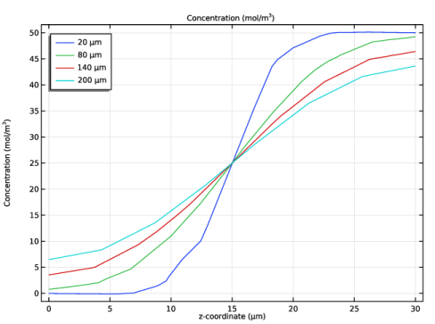
Click Replace Expression in the upper-right corner of the y-Axis Data section. From the menu, choose Component 1 (comp1)>Transport of Diluted Species>Species c>c - Concentration - mol/m³.
5
Click Replace Expression in the upper-right corner of the x-Axis Data section. From the menu, choose Component 1 (comp1)>Geometry>Coordinate>z - z-coordinate.
6
Click to expand the Legends section. Select the Show legends check box.
7
From the Legends list, choose Manual.
8
To enter the character ’µ’, copy the Unicode character u00b5 from an external tool (such as the Character Map in Windows) and paste into the table.
Line Graph 2
1
Right-click Line Graph 1 and choose Duplicate.
2
In the Settings window for Line Graph, locate the Data section.
3
From the Dataset list, choose Cut Line 3D 2.
4
Locate the Legends section. In the table, enter the following settings:
Line Graph 3
1
Right-click Line Graph 2 and choose Duplicate.
2
In the Settings window for Line Graph, locate the Data section.
3
From the Dataset list, choose Cut Line 3D 3.
4
Locate the Legends section. In the table, enter the following settings:
Line Graph 4
1
Right-click Line Graph 3 and choose Duplicate.
2
In the Settings window for Line Graph, locate the Data section.
3
From the Dataset list, choose Cut Line 3D 4.
4
Locate the Legends section. In the table, enter the following settings:
5
In the 1D Plot Group 5 toolbar, click  Plot.
Compare the result with Figure 5.
Appendix — Geometry Instructions
From the File menu, choose New.
New
In the New window, click  Blank Model.
Add Component
In the Home toolbar, click  Add Component and choose 3D.
Geometry 1
1
In the Settings window for Geometry, locate the Units section.
2
From the Length unit list, choose µm.
Block 1 (blk1)
1
In the Geometry toolbar, click  Block.
2
In the Settings window for Block, locate the Size and Shape section.
3
In the Width text field, type 80.
4
In the Depth text field, type 200.
5
In the Height text field, type 30.
6
Locate the Position section. In the y text field, type -200.
Work Plane 1 (wp1)
In the Geometry toolbar, click  Work Plane.
Work Plane 1 (wp1)>Plane Geometry
In the Model Builder window, click Plane Geometry.
Work Plane 1 (wp1)>Circle 1 (c1)
1
In the Work Plane toolbar, click  Circle.
2
In the Settings window for Circle, locate the Size and Shape section.
3
In the Radius text field, type 320.
4
In the Sector angle text field, type 90.
5
Locate the Position section. In the xw text field, type 320.
6
Locate the Rotation Angle section. In the Rotation text field, type 90.
7
Click to expand the Layers section. In the table, enter the following settings:
Work Plane 1 (wp1)>Rectangle 1 (r1)
1
In the Work Plane toolbar, click  Rectangle.
2
In the Settings window for Rectangle, locate the Size and Shape section.
3
In the Width text field, type 320.
4
In the Height text field, type 200.
Work Plane 1 (wp1)>Intersection 1 (int1)
1
In the Work Plane toolbar, click  Booleans and Partitions and choose Intersection.
2
Click in the Graphics window and then press Ctrl+A to select both objects.
3
In the Settings window for Intersection, click  Build Selected.
Work Plane 1 (wp1)>Delete Entities 1 (del1)
1
In the Work Plane toolbar, click  Delete.
2
In the Settings window for Delete Entities, locate the Entities or Objects to Delete section.
3
From the Geometric entity level list, choose Domain.
4
On the object int1, select Domains 2, 4, and 6 only.
Extrude 1 (ext1)
1
In the Model Builder window, under Component 1 (comp1)>Geometry 1 right-click Work Plane 1 (wp1) and choose Extrude.
2
In the Settings window for Extrude, locate the Distances section.
3
Copy 1 (copy1)
1
In the Geometry toolbar, click  Transforms and choose Copy.
2
3
In the Settings window for Copy, locate the Displacement section.
4
In the z text field, type 20.
Mirror 1 (mir1)
1
In the Geometry toolbar, click  Transforms and choose Mirror.
2
3
In the Settings window for Mirror, locate the Point on Plane of Reflection section.
4
In the x text field, type 40.
5
Locate the Normal Vector to Plane of Reflection section. In the x text field, type 1.
6
In the z text field, type 0.
Union 1 (uni1)
1
In the Geometry toolbar, click  Booleans and Partitions and choose Union.
2
Click in the Graphics window and then press Ctrl+A to select all objects.
3
In the Settings window for Union, locate the Union section.
4
Clear the Keep interior boundaries check box.
Form Union (fin)
1
In the Model Builder window, click Form Union (fin).
2
In the Settings window for Form Union/Assembly, click  Build Selected.
Geometry
1
In the Geometry toolbar, click  Selections and choose Explicit Selection.
2
On the object fin, select Domain 1 only.
3
In the Settings window for Explicit Selection, type Geometry in the Label text field.
All Walls
1
In the Geometry toolbar, click  Selections and choose Adjacent Selection.
2
In the Settings window for Adjacent Selection, type All Walls in the Label text field.
3
Locate the Input Entities section. Click  Add.
4
In the Add dialog box, select Geometry in the Input selections list.
5
Outlet
1
In the Geometry toolbar, click  Selections and choose Explicit Selection.
2
In the Settings window for Explicit Selection, type Outlet in the Label text field.
3
Locate the Entities to Select section. From the Geometric entity level list, choose Boundary.
4
On the object fin, select Boundary 16 only.
Concentration 1
1
In the Geometry toolbar, click  Selections and choose Explicit Selection.
2
In the Settings window for Explicit Selection, type Concentration 1 in the Label text field.
3
Locate the Entities to Select section. From the Geometric entity level list, choose Boundary.
4
On the object fin, select Boundaries 1, 6, and 11 only.
Concentration 2
1
In the Geometry toolbar, click  Selections and choose Explicit Selection.
2
In the Settings window for Explicit Selection, type Concentration 2 in the Label text field.
3
Locate the Entities to Select section. From the Geometric entity level list, choose Boundary.
4
On the object fin, select Boundaries 32, 35, and 36 only.
Inlet
1
In the Geometry toolbar, click  Selections and choose Union Selection.
2
In the Settings window for Union Selection, type Inlet in the Label text field.
3
Locate the Geometric Entity Level section. From the Level list, choose Boundary.
4
Locate the Input Entities section. Click  Add.
5
In the Add dialog box, in the Selections to add list, choose Concentration 1 and Concentration 2.
6
Symmetry
1
In the Geometry toolbar, click  Selections and choose Explicit Selection.
2
In the Settings window for Explicit Selection, type Symmetry in the Label text field.
3
Locate the Entities to Select section. From the Geometric entity level list, choose Boundary.
4
Select the Group by continuous tangent check box.
5
On the object fin, select Boundaries 4, 9, 14, 17, 18, 20, 26, and 30 only.
Exterior Walls
1
In the Geometry toolbar, click  Selections and choose Difference Selection.
2
In the Settings window for Difference Selection, type Exterior Walls in the Label text field.
3
Locate the Geometric Entity Level section. From the Level list, choose Boundary.
4
Locate the Input Entities section. Click  Add.
5
In the Add dialog box, select All Walls in the Selections to add list.
6
7
In the Settings window for Difference Selection, locate the Input Entities section.
8
9
In the Add dialog box, in the Selections to subtract list, choose Outlet, Inlet, and Symmetry.
10