PDF

Calibration Against TTT Data
Introduction
During component quenching, austenite decomposes into a combination of other phases such as ferrite, pearlite, bainite, and martensite. The final phase composition inside a quenched component depends on the thermal history during cooling, and also on the alloying of the steel itself. The variations in quenching characteristics between steels can be significant, and each steel has to be characterized with respect to how phase transformations occur during a thermal transient. A common way to illustrate the phase transformation characteristics is through transformation diagrams. Two of the most commonly used diagram types are the CCT (continuous cooling transformation) and the TTT (time-temperature transformation) diagrams. In the CCT case, the austenitized material is cooled at varying constant temperature rates, and fractions of the emerging phases formed are plotted as points in time-temperature space. In the TTT case, the material is first rapidly cooled, and than held at a constant temperature. Figure 1 shows a schematic of a TTT diagram, in which a single phase transformation is considered. It is customary to plot a curve denoting the start of formation of the destination phase, in this case when the destination phase reaches a fraction of 1%. In other words, the curve shows the time it takes, at a fixed temperature, to form 1% of the destination phase. To complete the diagram, other curves are typically included. In this example, the 50% and 90% curves are also drawn. When several curves are used, phase transformation models can be readily fitted for the isothermal case.
Figure 1: A TTT diagram.
In this model, TTT diagram data is used to calibrate the Johnson–Mehl–Avrami–Kolmogorov (JMAK) phase transformation model. Using the calibration result, a TTT diagram is computed and compared to the original TTT diagram data.
Model Definition
This model considers a set of experimental TTT data for a single phase transformation. The data is given in Table 1. The table shows, for each temperature, the times it takes to form 1%, 50%, and 90% of the phase.
In order to calibrate a phase transformation model to this experimental data, no geometry is required, and the temperature field can be replaced by a temperature parameter. For each temperature in Table 1, a least-squares problem is solved to find a set of phase transformation model parameters such that the evolution of the phase fraction matches the experimental data.
Phase Transformation
The model only considers a single phase transformation, and it is described by the JMAK model. This model requires three parameters:
In general, all these parameters can be used to calibrate the phase transformation against experimental data, but this model considers a special case where the phase fraction tends towards one, and where the Avrami exponent is considered constant and equal to three. For each temperature under consideration, the goal is to find the value of τ that produces the best least squares fit. The JMAK model is integrated using a time-dependent study step, and the phase fraction of the forming phase (the destination phase) can then be schematically expressed as ξ(t,τ), where t is time, and τ is the time constant.
Optimization
The purpose of the optimization, at a given temperature, is to find the optimal value for the phase transformation model parameter τ such that the phase fraction, that evolves over time, best reproduces the experimental data. An objective function can be expressed as
where the experimental data is given by N points, tk is the time at which ξk of the phase has formed. This objective function is minimized for each temperature to find τ.
Results and Discussion
The purpose of calibrating phase transformation models is to be able to use them to describe phase transformations that occur, for example, during component quenching. In this example, the JMAK phase transformation model was calibrated against TTT data. The result from the calibration procedure is the temperature-dependent parameter τ. The parameter is shown in Figure 2. The figure shows that the value of τ is high towards the ends of the temperature range, and smaller in the center of the range. The parameter τ represents a characteristic time for phase transformation, and the experimental data confirms that the phase transformation is most rapid at the intermediate temperatures. When the calibrated phase transformation model is used to compute a TTT diagram, you can compare the resulting diagram to the experimental (input) data. This is done in Figure 3. By merely using τ as a fitting parameter, the 1%, 50%, and 90% lines are reproduced well. For an even better fit to the experimental data, the Avrami exponent, here considered a constant, could be added as a free parameter of the optimization problem.
The methodology in this example can be used sequentially to calibrate several phase transformation models, one phase transformation at a time. A natural next step, once every relevant phase transformation has been characterized, is to simulate continuous cooling, and produce a CCT diagram. Good agreement between a computed CCT diagram with its experimental counterpart may require adjusting the phase transformation model parameters.
Figure 2: The temperature dependent phase transformation model parameter τ.
Figure 3: Comparison of the computed TTT diagram and experimental data, for the 1%, 50% and 90% lines.
Application Library path: Metal_Processing_Module/Transformation_Diagrams/calibration_against_ttt_data
Modeling Instructions
From the File menu, choose New.
New
In the New window, click  Model Wizard.
Model Wizard
1
In the Model Wizard window, click  0D.
2
In the Select Physics tree, select Heat Transfer>Metal Processing>Metal Phase Transformation (metp).
3
Click Add.
4
Click  Study.
5
In the Select Study tree, select General Studies>Time Dependent.
6
Global Definitions
Parameters 1
1
In the Model Builder window, under Global Definitions click Parameters 1.
2
In the Settings window for Parameters, locate the Parameters section.
3
Metal Phase Transformation (metp)
Metallurgical Phase 2
1
In the Model Builder window, under Component 1 (comp1)>Metal Phase Transformation (metp) click Metallurgical Phase 2.
2
In the Settings window for Metallurgical Phase, locate the Transformation Times section.
3
Select the Compute transformation times check box.
4
5
6
Phase Transformation 1
1
In the Model Builder window, click Phase Transformation 1.
2
In the Settings window for Phase Transformation, locate the Phase Transformation section.
3
From the Phase transformation model list, choose Johnson-Mehl-Avrami-Kolmogorov (JMAK).
4
In the ξeqd text field, type xieq.
5
In the τs −> d text field, type tau.
6
In the ns −> d text field, type n.
Component 1 (comp1)
In the Definitions toolbar, click  Optimization and choose Parameter Estimation>Global Least-Squares Objective.
Parameter Estimation
Global Least-Squares Objective 1
1
In the Settings window for Global Least-Squares Objective, locate the Experimental Data section.
2
In the Filename text field, type calibration_against_ttt_data_ttt001.txt.
3
Click  Import.
4
Locate the Column Settings section. In the table, click to select the cell at row number 1 and column number 3.
5
6
7
From the Name list, choose T (Temperature).
8
In the Unit text field, type K.
9
10
11
12
13
In the Model expression text field, type metp.phase2.xi.
14
In the Name text field, type col3a.
15
In the Weight text field, type 1/0.01^2.
Global Least-Squares Objective 2
1
Right-click Component 1 (comp1)>Parameter Estimation>Global Least-Squares Objective 1 and choose Duplicate.
2
In the Settings window for Global Least-Squares Objective, locate the Experimental Data section.
3
Find the Data imported into model subsection. Click Discard.
4
In the Filename text field, type calibration_against_ttt_data_ttt050.txt.
5
Click  Import.
6
Locate the Column Settings section. In the table, click to select the cell at row number 3 and column number 2.
7
In the Name text field, type col3b.
8
In the Weight text field, type 1/0.5^2.
Global Least-Squares Objective 3
1
Right-click Global Least-Squares Objective 2 and choose Duplicate.
2
In the Settings window for Global Least-Squares Objective, locate the Experimental Data section.
3
Find the Data imported into model subsection. Click Discard.
4
In the Filename text field, type calibration_against_ttt_data_ttt090.txt.
5
Click  Import.
6
Locate the Column Settings section. In the table, click to select the cell at row number 3 and column number 2.
7
In the Name text field, type col3c.
8
In the Weight text field, type 1/0.9^2.
Study 1
Step 1: Time Dependent
1
In the Model Builder window, under Study 1 click Step 1: Time Dependent.
2
In the Settings window for Time Dependent, locate the Study Settings section.
3
In the Output times text field, type range(0,50,28000).
4
From the Tolerance list, choose User controlled.
5
In the Relative tolerance text field, type 0.001.
6
Click to expand the Study Extensions section. Select the Auxiliary sweep check box.
7
8
Parametric Sweep
1
In the Study toolbar, click  Parametric Sweep.
2
In the Settings window for Parametric Sweep, locate the Study Settings section.
3
4
Parameter Estimation
1
In the Study toolbar, click  Optimization and choose Parameter Estimation.
2
In the Settings window for Parameter Estimation, locate the Experimental Data section.
3
From the Data source list, choose None.
4
Locate the Objective Function section. In the table, select the Active check boxes for Global Least-Squares Objective 1, Global Least-Squares Objective 2, and Global Least-Squares Objective 3.
5
Locate the Parameters section. Click  Add.
6
7
Locate the Parameter Estimation Method section. In the Optimality tolerance text field, type 0.0001.
8
In the Study toolbar, click  Compute.
Results
Parameter estimation, Parameter estimation 1, Parameter estimation 2
1
In the Model Builder window, under Results, Ctrl-click to select Parameter estimation, Parameter estimation 1, and Parameter estimation 2.
2
Evaluation Group 1
1
In the Results toolbar, click  Evaluation Group.
2
In the Settings window for Evaluation Group, locate the Data section.
3
From the Dataset list, choose Study 1/Parametric Solutions 1 (sol2).
4
From the Parameter selection (t, T) list, choose Last.
Global Evaluation 1
1
Right-click Evaluation Group 1 and choose Global Evaluation.
2
In the Settings window for Global Evaluation, locate the Expressions section.
3
4
In the Evaluation Group 1 toolbar, click  Evaluate.
You can now save the calibrated values into a text file, for example into a file called calibration_against_ttt_data_tau_calib.txt.
Table 1
1
In the Results toolbar, click  Data and choose Table.
2
In the Settings window for Table, locate the Table section.
3
From the Source list, choose Evaluation group.
4
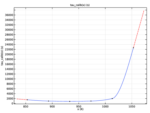
Locate the Output section. In the Filename text field, type calibration_against_ttt_data_tau_calib.txt.
Definitions
Interpolation 1 (int1)
1
In the Home toolbar, click  Functions and choose Local>Interpolation.
2
In the Settings window for Interpolation, locate the Definition section.
3
From the Data source list, choose File.
Assuming that the calibrated values for the phase transformation model have been stored in a file, the values can be imported as an interpolation function.
4
Click  Browse.
5
6
In the Number of arguments text field, type 1.
7
Find the Functions subsection. In the table, enter the following settings:
8
Locate the Interpolation and Extrapolation section. From the Interpolation list, choose Piecewise cubic.
9
From the Extrapolation list, choose Linear.
10
Locate the Units section. In the Argument table, enter the following settings:
11
In the Function table, enter the following settings:
12
13
Add Physics
1
In the Home toolbar, click  Add Physics to open the Add Physics window.
2
Go to the Add Physics window.
3
In the tree, select Recently Used>Metal Phase Transformation (metp).
4
Click Add to Component 1 in the window toolbar.
5
In the Home toolbar, click  Add Physics to close the Add Physics window.
Metal Phase Transformation 2 (metp2)
Metallurgical Phase 2
1
In the Model Builder window, under Component 1 (comp1)>Metal Phase Transformation 2 (metp2) click Metallurgical Phase 2.
2
In the Settings window for Metallurgical Phase, locate the Transformation Times section.
3
Select the Compute transformation times check box.
4
5
6
7
In the Model Builder window, click Metal Phase Transformation 2 (metp2).
8
In the Settings window for Metal Phase Transformation, locate the Temperature section.
9
In the T text field, type T.
Phase Transformation 1
1
In the Model Builder window, click Phase Transformation 1.
2
In the Settings window for Phase Transformation, locate the Phase Transformation section.
3
From the Phase transformation model list, choose Johnson-Mehl-Avrami-Kolmogorov (JMAK).
4
In the ξeqd text field, type xieq.
5
In the τs −> d text field, type tau_calib(metp2.T).
6
In the ns −> d text field, type n.
Add Study
1
In the Home toolbar, click  Add Study to open the Add Study window.
2
Go to the Add Study window.
3
Find the Studies subsection. In the Select Study tree, select General Studies>Time Dependent.
4
Click Add Study in the window toolbar.
5
In the Home toolbar, click  Add Study to close the Add Study window.
Study 2
Step 1: Time Dependent
1
In the Settings window for Time Dependent, locate the Study Settings section.
2
In the Output times text field, type range(0,25,28000).
3
From the Tolerance list, choose User controlled.
4
In the Relative tolerance text field, type 0.001.
5
Locate the Physics and Variables Selection section. In the table, clear the Solve for check box for Metal Phase Transformation (metp).
6
Locate the Study Extensions section. Select the Auxiliary sweep check box.
7
8
9
In the Home toolbar, click  Compute.
Results
Parameter estimation, Parameter estimation 1, Parameter estimation 2
1
In the Model Builder window, under Results, Ctrl-click to select Parameter estimation, Parameter estimation 1, and Parameter estimation 2.
2
Experiment (1%)
1
In the Model Builder window, expand the Results>Tables node.
2
Right-click Results>Tables and choose Table.
3
In the Settings window for Table, type Experiment (1%) in the Label text field.
4
Locate the Data section. Click Import.
5
Experiment (50%)
1
In the Results toolbar, click  Table.
2
In the Settings window for Table, type Experiment (50%) in the Label text field.
3
Locate the Data section. Click Import.
4
Experiment (90%)
1
In the Results toolbar, click  Table.
2
In the Settings window for Table, type Experiment (90%) in the Label text field.
3
Locate the Data section. Click Import.
4
1D Plot Group 3
1
In the Results toolbar, click  1D Plot Group.
2
In the Settings window for 1D Plot Group, locate the Data section.
3
From the Dataset list, choose Study 2/Solution 9 (sol9).
4
Locate the Plot Settings section. Select the x-axis label check box.
5
6
Select the y-axis label check box.
7
8
Locate the Axis section. Select the x-axis log scale check box.
9
Locate the Legend section. Clear the Show legends check box.
10
Click to expand the Title section. From the Title type list, choose Manual.
11
In the Title text area, type TTT diagram for 1%, 50% and 90% transformation.
Table Graph 1
1
Right-click 1D Plot Group 3 and choose Table Graph.
2
In the Settings window for Table Graph, locate the Data section.
3
From the Table list, choose Experiment (1%).
4
From the x-axis data list, choose Column 2.
5
From the Plot columns list, choose Manual.
6
In the Columns list, select Column 1.
7
Click to expand the Preprocessing section. Find the y-axis columns subsection. From the Preprocessing list, choose Linear.
8
In the Shift text field, type -273.15.
9
Locate the Coloring and Style section. Find the Line style subsection. From the Line list, choose None.
10
From the Color list, choose Magenta.
11
Find the Line markers subsection. From the Marker list, choose Asterisk.
12
From the Positioning list, choose In data points.
Table Graph 2
1
Right-click Table Graph 1 and choose Duplicate.
2
In the Settings window for Table Graph, locate the Data section.
3
From the Table list, choose Experiment (50%).
4
Locate the Coloring and Style section. From the Color list, choose Red.
Table Graph 3
1
Right-click Table Graph 2 and choose Duplicate.
2
In the Settings window for Table Graph, locate the Data section.
3
From the Table list, choose Experiment (90%).
4
Locate the Coloring and Style section. From the Color list, choose Blue.
Global 1
1
In the Model Builder window, right-click 1D Plot Group 3 and choose Global.
2
In the Settings window for Global, locate the y-Axis Data section.
3
Click  Clear Table.
4
5
Locate the x-Axis Data section. From the Parameter list, choose Expression.
6
In the Expression text field, type metp2.phase2.time_1.
7
Click to expand the Coloring and Style section. From the Color list, choose Magenta.
8
Set the Width value to 3.
Global 2
1
Right-click Global 1 and choose Duplicate.
2
In the Settings window for Global, locate the y-Axis Data section.
3
4
Locate the x-Axis Data section. In the Expression text field, type metp2.phase2.time_2.
5
Locate the Coloring and Style section. From the Color list, choose Red.
Global 3
1
Right-click Global 2 and choose Duplicate.
2
In the Settings window for Global, locate the y-Axis Data section.
3
4
Locate the x-Axis Data section. In the Expression text field, type metp2.phase2.time_3.
5
Locate the Coloring and Style section. From the Color list, choose Blue.
1D Plot Group 3
1
In the Model Builder window, click 1D Plot Group 3.
2
In the Settings window for 1D Plot Group, locate the Data section.
3
From the Time selection list, choose Last.
4
In the 1D Plot Group 3 toolbar, click  Plot.
Annotation 1
1
Right-click 1D Plot Group 3 and choose Annotation.
2
In the Settings window for Annotation, locate the Annotation section.
3
In the Text text field, type 1% (computed).
4
Locate the Position section. In the x text field, type 5000.
5
In the y text field, type 700.
6
Locate the Coloring and Style section. From the Color list, choose Magenta.
Annotation 2
1
Right-click Annotation 1 and choose Duplicate.
2
In the Settings window for Annotation, locate the Annotation section.
3
In the Text text field, type 50% (computed).
4
Locate the Coloring and Style section. From the Color list, choose Red.
5
Locate the Position section. In the y text field, type 680.
Annotation 3
1
Right-click Annotation 2 and choose Duplicate.
2
In the Settings window for Annotation, locate the Annotation section.
3
In the Text text field, type 90% (computed).
4
Locate the Coloring and Style section. From the Color list, choose Blue.
5
Locate the Position section. In the y text field, type 660.
6
In the 1D Plot Group 3 toolbar, click  Plot.