|
|
|
|
1
|
|
2
|
|
3
|
Click Add.
|
|
4
|
Click
|
|
5
|
|
6
|
Click
|
|
1
|
|
2
|
|
3
|
|
1
|
|
2
|
|
3
|
|
4
|
Browse to the model’s Application Libraries folder and double-click the file squeeze_film_perforated_plates_parameters.txt.
|
|
1
|
|
2
|
|
3
|
|
4
|
|
1
|
|
2
|
|
3
|
|
4
|
|
5
|
|
6
|
|
1
|
|
1
|
|
2
|
In the Settings window for Thin-Film Flow, Domain, type Thin-Film Flow, Domain - no perforation in the Label text field.
|
|
3
|
|
4
|
|
1
|
In the Model Builder window, under Component 1 (comp1)>Thin-Film Flow, Domain - no perforation (tff) click Fluid-Film Properties 1.
|
|
2
|
|
3
|
|
4
|
|
1
|
|
2
|
|
3
|
|
4
|
|
5
|
|
1
|
In the Settings window for Thin-Film Flow, Domain, type Thin-Film Flow, Domain - Bao model in the Label text field.
|
|
2
|
|
3
|
|
1
|
In the Model Builder window, under Component 1 (comp1)>Thin-Film Flow, Domain - Bao model (tff2) click Fluid-Film Properties 1.
|
|
2
|
|
3
|
|
4
|
|
1
|
|
3
|
|
4
|
|
5
|
|
6
|
|
7
|
|
1
|
|
2
|
|
3
|
|
1
|
|
2
|
|
1
|
|
2
|
In the Settings window for Interpolation, type Interpolation of experimental data in the Label text field.
|
|
3
|
|
4
|
Click
|
|
5
|
Browse to the model’s Application Libraries folder and double-click the file squeeze_film_perforated_plates_exp_data.txt.
|
|
6
|
Click
|
|
7
|
Locate the Interpolation and Extrapolation section. From the Interpolation list, choose Nearest neighbor.
|
|
8
|
|
9
|
In the Function table, enter the following settings:
|
|
1
|
|
2
|
|
1
|
|
2
|
|
3
|
|
4
|
|
1
|
|
2
|
|
3
|
|
4
|
|
5
|
|
1
|
|
2
|
Select the object sq1 only.
|
|
3
|
|
4
|
|
5
|
|
6
|
|
7
|
|
8
|
Locate the Selections of Resulting Entities section. Select the Resulting objects selection check box.
|
|
1
|
|
2
|
Select the object r1 only.
|
|
3
|
|
4
|
|
5
|
|
1
|
|
2
|
|
3
|
|
4
|
|
5
|
|
1
|
In the Settings window for Thin-Film Flow, Domain, type Thin-Film Flow, Domain - P = 0 at perf in the Label text field.
|
|
2
|
|
3
|
|
1
|
In the Model Builder window, under Component 2 (comp2)>Thin-Film Flow, Domain - P = 0 at perf (tff3) click Fluid-Film Properties 1.
|
|
2
|
|
3
|
|
4
|
|
1
|
|
2
|
|
3
|
|
1
|
|
2
|
|
1
|
|
2
|
|
3
|
|
4
|
Browse to the model’s Application Libraries folder and double-click the file squeeze_film_perforated_plates_study_data.txt.
|
|
1
|
|
2
|
|
3
|
|
4
|
|
1
|
|
1
|
|
2
|
|
1
|
|
2
|
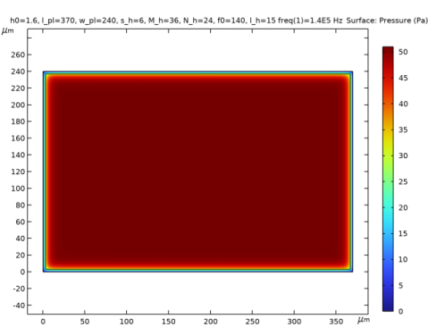
In the Settings window for 2D Plot Group, type 2D Plot Group 3 - P=0 at perf in the Label text field.
 |
|
1
|
|
2
|
|
3
|
|
4
|
|
5
|
|
6
|
|
7
|
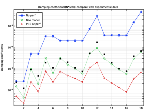
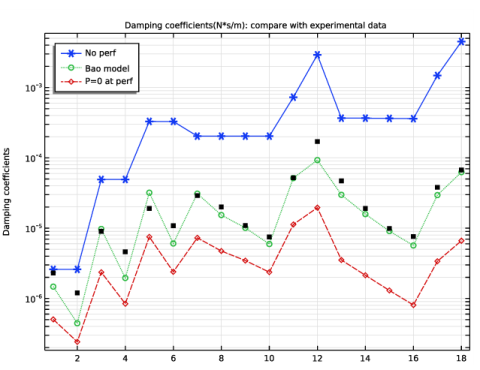
In the associated text field, type Damping coefficients.
|
|
8
|
|
9
|
|
1
|
|
2
|
|
4
|
|
5
|
Click to expand the Coloring and Style section. Find the Line style subsection. From the Line list, choose Cycle.
|
|
6
|
|
7
|
|
1
|
|
2
|
|
3
|
|
4
|
|
1
|
In the Model Builder window, under Component 1 (comp1)>Definitions click Interpolation of experimental data (int1).
|
|
2
|
|
1
|
|
2
|
|
3
|
|
4
|
|
1
|
|
2
|
|
3
|
|
4
|
|
5
|
|
6
|