|
|
|


|
1
|
|
2
|
|
3
|
Click Add.
|
|
4
|
Click
|
|
5
|
|
6
|
Click
|
|
1
|
|
2
|
|
1
|
|
2
|
|
3
|
|
4
|
|
5
|
|
6
|
|
7
|
|
1
|
|
2
|
|
3
|
|
1
|
|
2
|
|
1
|
|
2
|
|
3
|
|
4
|
|
5
|
Locate the Units section. In the table, enter the following settings:
|
|
6
|
|
1
|
In the Model Builder window, under Component 1 (comp1) right-click Materials and choose Blank Material.
|
|
2
|
|
1
|
|
2
|
|
3
|
|
1
|
In the Model Builder window, under Component 1 (comp1)>Thin-Film Flow, Edge (tffs) click Fluid-Film Properties 1.
|
|
2
|
In the Settings window for Fluid-Film Properties, click to expand the Reference Surface Properties section.
|
|
3
|
|
4
|
|
5
|
|
6
|
|
1
|
Right-click Component 1 (comp1)>Thin-Film Flow, Edge (tffs)>Fluid-Film Properties 1 and choose Duplicate.
|
|
3
|
|
4
|
|
5
|
|
1
|
|
2
|
|
3
|
|
4
|
|
5
|
|
1
|
|
2
|
|
3
|
|
4
|
Locate the Physics and Variables Selection section. Select the Modify model configuration for study step check box.
|
|
5
|
|
6
|
Right-click and choose Disable.
|
|
7
|
|
8
|
|
1
|
|
2
|
|
3
|
|
4
|
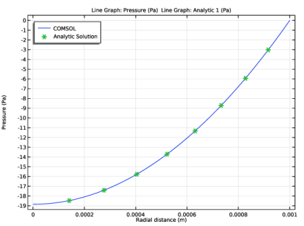
In the associated text field, type Radial distance (m).
|
|
5
|
|
6
|
In the associated text field, type Pressure (Pa).
|
|
7
|
|
1
|
|
3
|
|
4
|
|
5
|
|
1
|
|
3
|
|
4
|
|
5
|
Click to expand the Coloring and Style section. Find the Line style subsection. From the Line list, choose None.
|
|
6
|
|
7
|
|
8
|
|
10
|
|
11
|
|
1
|
|
2
|
|
3
|
Click OK.
|
|
1
|
|
2
|
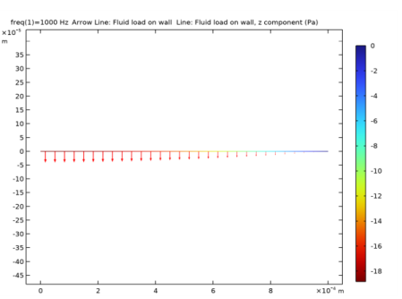
In the Settings window for Arrow Line, click Replace Expression in the upper-right corner of the Expression section. From the menu, choose Component 1 (comp1)>Thin-Film Flow, Edge>Fluid loads>tffs.fwallr,tffs.fwallz - Fluid load on wall.
|
|
3
|
|
4
|
|
6
|
|
7
|
|
1
|
|
2
|
In the Settings window for Line, click Replace Expression in the upper-right corner of the Expression section. From the menu, choose Component 1 (comp1)>Thin-Film Flow, Edge>Fluid loads>Fluid load on wall - N/m²>tffs.fwallz - Fluid load on wall, z component.
|
|
3
|
|
4
|
|
5
|
|
1
|
|
2
|
|
3
|
Click OK.
|
|
1
|
|
2
|
|
4
|
Click
|
|
1
|
|
2
|
In the Settings window for Global Evaluation, click Replace Expression in the upper-right corner of the Expressions section. From the menu, choose Component 1 (comp1)>Definitions>Variables>Ftotan - Analytic expression - N.
|
|
3
|
|
1
|
|
2
|
|
3
|
|
4
|
|
5
|
|
1
|
|
2
|
Click
|
|
3
|
|
4
|
|
5
|
Click Replace.
|
|
6
|
|
7
|
|
8
|
Click
|
|
10
|
|
1
|
|
2
|
|
3
|
|
1
|
|
3
|
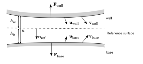
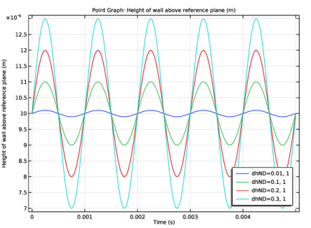
In the Settings window for Point Graph, click Replace Expression in the upper-right corner of the y-Axis Data section. From the menu, choose Component 1 (comp1)>Thin-Film Flow, Edge>Wall and base properties>tffs.hw - Height of wall above reference plane - m.
|
|
4
|
|
5
|
|
1
|
|
2
|
|
3
|
|
4
|
|
5
|
|
6
|
|
7
|
|
8
|
|
9
|
Click OK.
|
|
10
|
|
11
|
|
1
|
|
2
|
|
3
|
|
1
|
|
3
|
|
1
|
|
2
|
|
3
|
Click OK.
|
|
4
|
|
5
|
|
1
|
|
3
|
|
5
|
Click
|
|
1
|
|
2
|
|
3
|
|
4
|
|
5
|
|
7
|
|
8
|
Click
|
|
1
|
Go to the Table window.
|
|
1
|
|
2
|
|
3
|
|
1
|
|
2
|
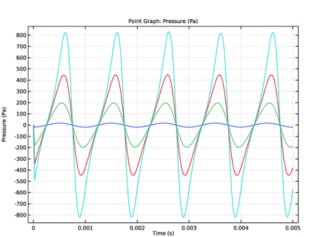
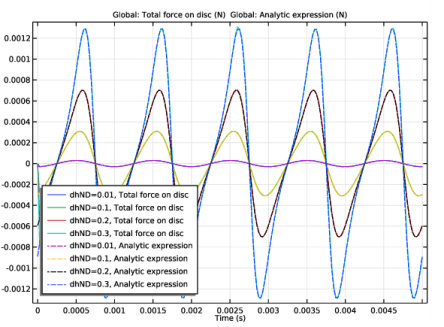
In the Settings window for Global, click Replace Expression in the upper-right corner of the y-Axis Data section. From the menu, choose Component 1 (comp1)>Definitions>Variables>Ftot - Total force on disc - N.
|
|
1
|
|
2
|
In the Settings window for Global, click Replace Expression in the upper-right corner of the y-Axis Data section. From the menu, choose Component 1 (comp1)>Definitions>Variables>Ftotantime - Analytic expression - N.
|
|
3
|
Click to expand the Coloring and Style section. Find the Line style subsection. From the Line list, choose Dashed.
|
|
1
|
|
2
|
|
3
|
|
4
|
|
5
|
|
6
|
|
7
|
|
8
|
In the Rename 1D Plot Group dialog box, type Total force on disc vs. time in the New label text field.
|
|
9
|
Click OK.
|
|
10
|
|
11
|